The previous two chapters gave two views of the same objective. This chapter builds variants of it. Recall:
In the general case, this means solving two optimization problems. First we find all the models that make the best predictions; then, among those, we pick the one with the smallest weights. Writing down a closed form for this takes more advanced linear algebra (the singular value decomposition). Instead, we change the objective so that both criteria live in a single objective.
That is the idea of regularization: \[ \text{regularized loss} := \text{prediction quality} + \text{"model complexity"}. \]
The first term measures how well the model fits the data; it was the only term in OLS. The second builds in a preference for some parameters over others. If two models fit the data equally well, there is no reason to choose the more complex one. Complex models tend to overfit (we make this precise in the regression recap), while simpler models tend to generalize better to unseen data.
The first term is the same total squared error as in OLS. The second adds the objective of the secondary problem above, the squared norm of the weights, directly into the loss. The scaling \(\lambda\) lets us choose how much we care about it.
Both \(w\) and \(\lambda\) are unknown, but they play different roles. The parameters \(w\) are fitted to the data. The hyperparameter \(\lambda\) is chosen before fitting, and it says how heavily to penalize model complexity. How do we choose it? One common answer, cross-validation, comes at the end of this chapter.
The ridge loss is still convex and differentiable, so we take the gradient and set it to zero. First rewrite the penalty in a form our gradient table handles: \[ \lambda \|w\|^2 = \lambda\, w^\top w = \lambda\, w^\top I w. \] (Check for yourself that putting the identity matrix between \(w^\top\) and \(w\) changes nothing.) Using \(\nabla(w^\top B w) = 2Bw\) with \(B = \lambda I\), and the OLS gradient from Chapter 1.1, \[ \begin{aligned} L_{\text{ridge}}(w) &= \|Xw - y\|^2 + \lambda\, w^\top I w \\ \Rightarrow\quad \nabla L_{\text{ridge}}(w) &= 2X^\top X w - 2X^\top y + 2\lambda I w \\ \Rightarrow\quad 2X^\top X\, w_{\text{ridge}} - 2X^\top y + 2\lambda I\, w_{\text{ridge}} &= 0 \\ \Rightarrow\quad X^\top X\, w_{\text{ridge}} + \lambda I\, w_{\text{ridge}} &= X^\top y \\ \Rightarrow\quad (X^\top X + \lambda I)\, w_{\text{ridge}} &= X^\top y. \end{aligned} \] Unlike \(X^\top X\), the matrix \(X^\top X + \lambda I\) is always invertible when \(\lambda > 0\), so \[ w_{\text{ridge}} := \operatorname*{argmin}_w \big(\|Xw - y\|^2 + \lambda \|w\|^2\big) = (X^\top X + \lambda I)^{-1} X^\top y. \]
Suppose \(w_1\) and \(w_2\) are two candidate weights with \(\|Xw_1 - y\| > \|Xw_2 - y\|\) (so \(w_2\) fits the data better), but \(\|w_1\| < \|w_2\|\) (so \(w_1\) is simpler). Which one does ridge prefer?
It depends on \(\lambda\). A large \(\lambda\) says model simplicity matters more than prediction quality, so it favors \(w_1\). A small \(\lambda\) favors the better fit, \(w_2\). If you strongly believe the true model should be simple, choose a larger \(\lambda\). If you are less sure, start with a smaller one.
Why is a small norm “simple”? Suppose two sets of weights make equally good predictions, but one has much larger entries. The model with smaller weights is more stable: a small change in the input causes only a small change in the output. With large weights, a tiny change in the input can change the output a lot.
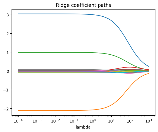
Does ridge ever set a weight to exactly zero? Generally, no. The ridge objective is smooth, so as \(\lambda\) grows the learned weights shrink smoothly toward zero without abruptly landing on it. We will see this in the demo below.
The squared norm is one way to measure model complexity, but it is not the only one. To describe others, we generalize the norm.
Definition. Given \(p \geq 1\), the \(\ell_p\)-norm of a vector \(w \in \mathbb{R}^d\) is \[ \|w\|_p := \Big(\sum_{j=1}^d |w_j|^p\Big)^{1/p}. \] (We index by \(j\) because we are summing over feature dimensions, not data points.) Take the absolute value of each entry, raise it to the power \(p\), sum, and take the \(p\)-th root to normalize.
Examples.
The squared norm we have been using all along is the squared \(\ell_2\)-norm, which is why the ridge objective above writes \(\|\cdot\|_2^2\).
We still measure prediction quality with the squared \(\ell_2\)-norm, but now we measure model complexity with the \(\ell_1\)-norm: the sum of the absolute values of the weights, instead of the sum of their squares.
Why not square the \(\ell_1\) term? We squared the \(\ell_2\)-norm because that removes its square root. The \(\ell_1\)-norm has no square root to remove. You could square it, but the unsquared version is the one used in practice. It is a design choice.
There is no closed-form solution. The reason is the absolute value: in one dimension, \(|w|\) has a sharp corner at \(0\), so the objective is not differentiable everywhere, and the “set the gradient to zero” approach no longer applies. A minimizer still exists, and in practice we find it with an iterative algorithm.
You might expect lasso to behave like ridge, shrinking weights toward zero. It does, but it also does something more surprising: it strongly prefers weights that are exactly zero. Lasso, or \(\ell_1\)-regularization, encourages sparse solutions, in which many weights are exactly \(0\).
The intuition for why is not obvious; it can be explained with tools from convex optimization. Here we will simply see it happen in the demo.
Sparsity makes lasso models more interpretable. A good model should not only make good predictions; ideally it also teaches us something about the world. The features whose weights lasso leaves non-zero are the ones that actually matter for prediction.
We simulate \(n = 100\) data points with \(d = 20\) features (ignoring the bias for simplicity), where only the first three features matter. We generate labels the same way as the generative model in Chapter 1.2: a linear prediction plus Gaussian noise.
import numpy as np
from sklearn.linear_model import Ridge, Lasso

np.random.seed(0)
n, d = 100, 20
X = np.random.randn(n, d)

w_true = np.zeros(d)
w_true[:3] = [3, -2, 1]            # only the first 3 features matter
y = X @ w_true + 0.5 * np.random.randn(n)

lambdas = np.logspace(-4, 3, 50)   # 50 values from 1e-4 to 1e3

ridge_coefs = np.array([Ridge(alpha=lam).fit(X, y).coef_ for lam in lambdas])
lasso_coefs = np.array([Lasso(alpha=lam, max_iter=5000).fit(X, y).coef_ for lam in lambdas])
In scikit-learn, the hyperparameter is called alpha; it
plays the role of our \(\lambda\). Each
of the resulting arrays has shape \(50 \times
20\): one row per \(\lambda\),
one column per weight. Plotting each column against \(\lambda\) shows how each learned weight
changes as the penalty grows.
Ridge. As \(\lambda\) increases, every weight shrinks toward zero, as expected. But even at \(\lambda = 10^3\), a very strong penalty given that the labels are smaller than 10 in magnitude, the weights are close to zero but none is exactly zero.
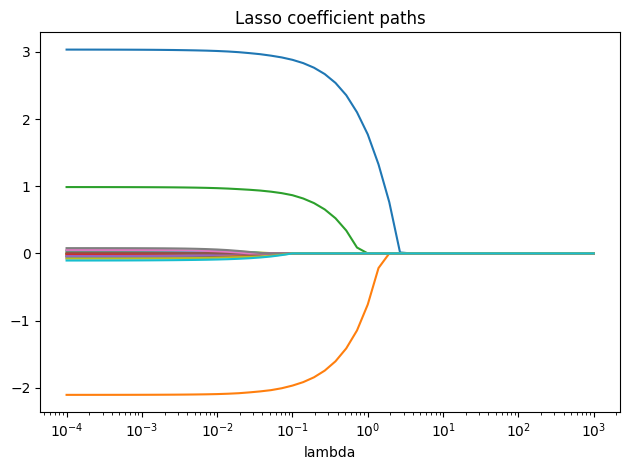
Lasso. The picture is different. As \(\lambda\) grows, the 17 irrelevant weights are pulled to exactly zero, with an almost abrupt transition, while the three true features stay non-zero. In that range, lasso has recovered the true model. As \(\lambda\) keeps increasing, even those three are eventually pulled to zero, and at the largest \(\lambda\) every weight is exactly zero.
Ridge minimizes exactly our ridge objective.
Lasso minimizes \(\frac{1}{2n}\|Xw - y\|_2^2 + \alpha
\|w\|_1\), so its alpha corresponds to a rescaled
\(\lambda\). The qualitative picture is
the same.
How do we pick the hyperparameter \(\lambda\)? In general, it is hard to know the best value in advance. A standard approach is \(K\)-fold cross-validation:
There is no universally right range of candidates. A log-spaced grid like the one above is a reasonable default, and in practice you may need to try a few.
The held-out group in each round acts as a validation set: a small slice of the training data, set aside to play the role of unseen test data. Repeating this \(K\) times, holding out a different slice each time, gives an estimate that is more robust than relying on a single split.
Remarks.
The regression recap discusses a cheaper version of this workflow that is common when datasets are large.