Last time we covered:
A follow-up on one question from Chapter 1.3: why not regularize with the squared \(\ell_1\)-norm? You could, and the resulting problem can still be solved iteratively, but squaring the \(\ell_1\) term loses the sparsity that makes lasso useful. Try it in code and compare the coefficient paths. Many choices in machine learning are like this: design choices that have proven useful in practice.
This chapter has two goals:
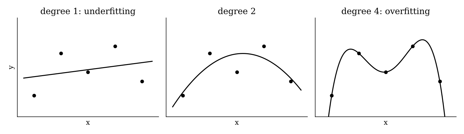
Suppose someone collects five data points with one feature each, and we fit three different models.
Most people would deploy the middle one. The rest of the first half of this chapter makes these intuitions precise.
We have only fit linear models so far, but you already know how to fit the other two. Transform the features nonlinearly, for example \(x \mapsto (x, x^2, x^3, x^4)\), then fit a linear model on the transformed features with OLS. This is polynomial regression. It models a nonlinear relationship, but it is still a linear model, because it is linear in the parameters \(w\).
How do we reason about the prediction error of a trained model?
What is random in \((\hat f(x) - Y)^2\)? Both terms. We have fixed the input \(x\), but \(\hat f\) is still random, because the training data are random. And \(Y\) is random, because the measurement itself is noisy. The two terms are random for different reasons.
We fix \(x\) because otherwise there are too many sources of randomness to untangle. With \(x\) fixed, the error splits into interpretable pieces. To reason about error over the whole input space, take a further expectation over \(X\).
Definition. At \(X = x\):
In the bias and variance, the expectation is over the randomness in the training data \(D\). \(\mathbb{E}[\hat f(x)]\) is the average prediction at \(x\) over all the datasets we might have collected.
Remarks.
\[ \text{expected prediction error} = \text{bias}^2 + \text{variance} + \text{noise}. \]
The proof is a direct, if not very interesting, calculation; try it if you like. What matters is the consequence. To reduce the error on future data, we need to reduce these three terms. The noise is out of our control. Bias and variance, however, depend on our choice of model class and learning algorithm.
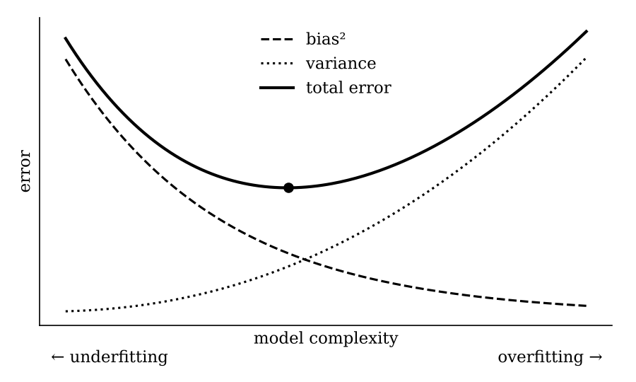
Think of fitting polynomials of increasing degree.
The total error is their sum (plus the noise), and the goal is the sweet spot in between. Models to the left of it, with high error from too little complexity, are underfitting. Models to the right, with high error from too much complexity, are overfitting. Model selection, whether with a validation set or cross-validation, is a search for that sweet spot along the complexity axis.
For ridge and lasso, what happens to the bias and the variance as \(\lambda\) increases?
One source of error goes up while the other goes down. That is exactly why choosing a hyperparameter is a balancing act.
The framework above suggests a direct approach: why not estimate \[ f^*(x) := \mathbb{E}[Y \mid X = x] \] itself? If we knew the joint distribution of \(X\) and \(Y\), we could compute it exactly, but estimating that distribution is hard. The formula is also not directly usable on data: at a particular \(x\), we may not have a single training point with exactly that input.
The idea of kernel regression is a locality assumption: the output changes smoothly with the input. To predict at \(x\), look at training points whose inputs are close to \(x\), and take a weighted average of their labels: \[ \hat f(x) := \sum_{i=1}^n w(x, x_i)\, y_i, \] where the weights \(w(x, x_i)\) are higher for local observations. Labels of nearby points are more informative than labels of distant ones. The remaining question is how to define good weights, and that is what kernels are for.
Definition. A function \(K : \mathbb{R} \to \mathbb{R}\) is called a localization kernel if it satisfies:
Remark. In kernel regression, we use \(K(x_1 - x_2)\) to measure the closeness of \(x_1\) and \(x_2\). Think of a kernel as the opposite of a distance: it is large when two points are close. So we want the kernel to have its mass concentrated near \(u = 0\).
This explains the first two properties. Closeness should be non-negative. And it should be symmetric: how close \(x_1\) is to \(x_2\) is the same as how close \(x_2\) is to \(x_1\). The last two properties are technical. They are convenient for proving theoretical results about kernel regression.
Examples.
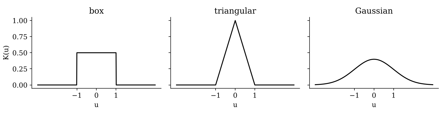
Why should “close” mean within distance 1? We can rescale any kernel to change the size of the neighborhood.
Definition. Given a kernel \(K\) and a bandwidth \(h > 0\), the scaled kernel is \[ K_h(u) := \frac1h K\!\Big(\frac uh\Big). \] Dividing the input by \(h\) stretches the neighborhood. The factor \(\frac1h\) keeps \(K_h\) integrating to 1. In practice that factor doesn’t matter, because kernel regression normalizes the weights anyway.
Example. For the box kernel, \(K_1\) equals \(\tfrac12\) on \([-1, 1]\), while \(K_{10}\) equals \(\tfrac{1}{20}\) on \([-10, 10]\): a neighborhood ten times wider, at a twentieth of the height.
The kernel turns a distance into a closeness score, and the denominator normalizes the scores so that the weights sum to 1. The prediction is a weighted average of the training labels.
To generalize to \(d\)-dimensional features, replace the difference \(x - x_i\) with the distance \(\|x - x_i\|_2\) as the input to the kernel.
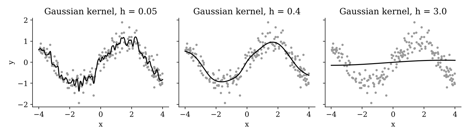
Both hyperparameters control model complexity. The bandwidth is the more important knob. A small \(h\) averages over very few neighbors and follows the noise, giving low bias and high variance. A large \(h\) averages over almost everything and flattens the curve, giving high bias and low variance.
Recall that we wanted to estimate \(f^*(x) = \mathbb{E}[Y \mid X = x]\). Kernel regression does so in the limit. For most kernels, including all the ones above, if \[ n \to \infty, \qquad h \to 0, \qquad nh \to \infty, \] then the kernel regression estimator converges to \(f^*(x) := \mathbb{E}[Y \mid X = x]\).
In words: as we collect more data, we can trust smaller neighborhoods, so the bandwidth shrinks. But the amount of data must grow faster than the neighborhood shrinks, so that each neighborhood still contains many points.
This is a beautiful result. In theory, kernel regression is as good as it gets. Yet it is not widely used in practice.
Why might kernel regression not be widely used, despite this guarantee?
The regression recap ties these together.