This chapter ties the regression module together. It adds two practical pieces we have not written down yet: the train/validation/test workflow used in practice, and how training and test error behave as models get more complex. It then summarizes every model in the module, and ends with practice problems.
Chapter 1.3 introduced \(K\)-fold cross-validation as the classical way to choose hyperparameters. It is the standard statistical framework, but with large datasets, training even one model can be expensive, and repeating it \(K\) times for every candidate is often not worth the cost. In practice, a cheaper version is common:
Compare this with cross-validation. Cross-validation repeats steps 1–2 over \(K\) different splits to get a more reliable error estimate. The workflow above does it once.
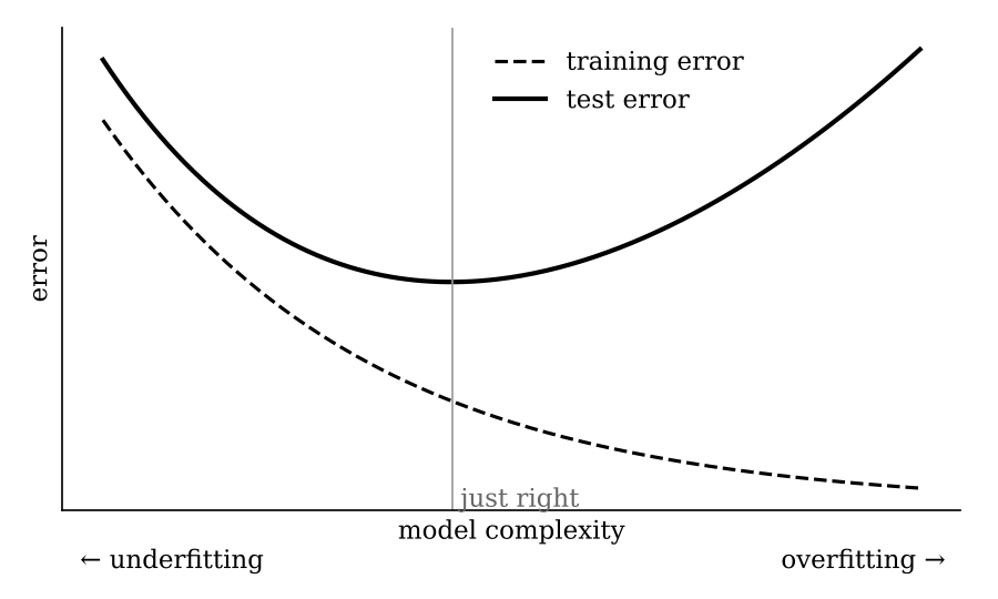
As model complexity increases, for example as we raise the polynomial degree or lower the regularization strength:
Model selection looks for the sweet spot in the middle. To the left, the model is underfitting: too simple to capture the data. To the right, it is overfitting: so complex that it fits the noise.
The bias–variance decomposition from Chapter 1.4 explains this curve: \[ \mathbb{E}\big[(\hat f(x) - Y)^2 \mid X = x\big] = \underbrace{\big(\mathbb{E}[\hat f(x)] - f^*(x)\big)^2}_{\text{bias}^2} + \underbrace{\mathbb{E}\big[(\hat f(x) - \mathbb{E}[\hat f(x)])^2\big]}_{\text{variance}} + \underbrace{\mathbb{E}\big[(Y - f^*(x))^2 \mid X = x\big]}_{\text{noise}}. \]
Increasing complexity usually lowers bias and raises variance. Their sum is the U-shaped test error. For every model in this course, ask yourself: how does this knob move bias and variance?
Recall the supervised learning pipeline from the Introduction. We assume there is a relatively simple function \(f^*\) with \(f^*(x_i) \approx y_i\). Under a generative model, a natural candidate is \(f^*(x) = \mathbb{E}[Y \mid X = x]\). Given \(n\) samples, the learning task is to find \(\hat f \approx f^*\) that makes mostly correct predictions on unseen data.
Every method in this module made the same two choices:
Yes. Polynomial regression models a nonlinear relationship between input and output, but “linear model” refers to linearity in the parameters. Since \(f(x) = w \cdot \phi(x)\) is linear in \(w\), polynomial regression is a linear model on nonlinear features. Every parametric model in this module is linear in this sense. Truly nonlinear models come later in the course.
For \(k = 1\), the transformation \(\phi\) just appends a 1 to each input. That is exactly bias lifting, so OLS is polynomial regression of degree 1.
The penalty moves the model toward the simpler, left side of the complexity curve. Because \(X^\top X + \lambda I\) is always invertible for \(\lambda > 0\), no pseudo-inverse is needed, and ridge solutions tend to be more stable. Regularization is a general idea: you can regularize polynomial regression the same way.
Practice each of these without looking at the notes:
The only formulas you need to bring are: \[ f(w) = w^\top B \;\Rightarrow\; \nabla f(w) = B, \qquad f(w) = w^\top B w \;\Rightarrow\; \nabla f(w) = 2Bw \;\; (B \text{ symmetric}), \] and the density of a 1-d Gaussian with mean \(\mu\) and variance \(\sigma^2\), \[ X \sim \mathcal{N}(\mu, \sigma^2) \;\Rightarrow\; p(x) = \frac{1}{\sqrt{2\pi\sigma^2}} \exp\!\Big(-\frac{(x - \mu)^2}{2\sigma^2}\Big). \]
These problems are in the style of the module assessment: a mix of short derivations and conceptual questions. Try each one before opening its solution.
Given data \((x_1, y_1), \dots, (x_n, y_n) \in \mathbb{R} \times \mathbb{R}\) with not all \(x_i = 0\), fit the model \(f(x) = wx\) (no bias) by minimizing \(L(w) = \sum_{i=1}^n (w x_i - y_i)^2\). Find \(\hat w\) in terms of the data.
\(L'(w) = \sum_i 2x_i(w x_i - y_i)\). Setting it to zero gives \[ \hat w = \frac{\sum_{i=1}^n x_i y_i}{\sum_{i=1}^n x_i^2}. \] \(L\) is a convex quadratic in \(w\), so this stationary point is the global minimizer. As a check, this is the matrix formula \((X^\top X)^{-1} X^\top y\) with \(X\) a single column: \(X^\top X = \sum_i x_i^2\) and \(X^\top y = \sum_i x_i y_i\).
In Chapter 1.2 we assumed \(\varepsilon_i \sim \mathcal{N}(0, 1)\). Suppose instead \(\varepsilon_i \sim \mathcal{N}(0, \sigma^2)\) for a known \(\sigma^2 > 0\). Show that the maximum likelihood estimate of \(w\) is still \(w_{\text{OLS}}\).
Now \(Y_i \sim \mathcal{N}(w^\top x_i, \sigma^2)\), so \[ \log p(y_i) = -\tfrac12 \log(2\pi\sigma^2) - \frac{1}{2\sigma^2}(y_i - w^\top x_i)^2, \quad\text{and}\quad \sum_{i=1}^n \log p(y_i) = -\frac{1}{2\sigma^2}\|Xw - y\|^2 + \text{constant}. \] Dropping the constant and the positive factor \(\frac{1}{2\sigma^2}\) does not change the argmax, so maximizing the log-likelihood is the same as minimizing \(\|Xw - y\|^2\). This is the claim from Chapter 1.2 that a general variance “gives the same result.”
Using the setup of Problem 1, minimize \(L(w) = \sum_i (w x_i - y_i)^2 + \lambda w^2\) for \(\lambda > 0\). Compare your answer with Problem 1. What happens as \(\lambda \to 0\) and as \(\lambda \to \infty\)?
Setting \(L'(w) = \sum_i 2x_i(w x_i - y_i) + 2\lambda w = 0\) gives \[ \hat w_{\text{ridge}} = \frac{\sum_i x_i y_i}{\sum_i x_i^2 + \lambda}. \] The denominator is larger than in Problem 1, so \(|\hat w_{\text{ridge}}| < |\hat w_{\text{OLS}}|\) whenever \(\hat w_{\text{OLS}} \neq 0\). Ridge shrinks the weight toward zero.
Training data: \((0, 1), (1, 3), (2, 2), (4, 10)\). Use the box kernel with bandwidth \(h = 1\).
With the box kernel and \(h = 1\), \(K_1(x - x_i) = \tfrac12\) if \(|x - x_i| \leq 1\) and \(0\) otherwise. So the prediction is the plain average of the labels of training points within distance 1.
Within distance 1 of \(1.5\): \(x_i = 1\) and \(x_i = 2\). So \(\hat f(1.5) = (3 + 2)/2 = 2.5\).
Within distance 1 of \(3\): \(x_i = 2\) and \(x_i = 4\). So \(\hat f(3) = (2 + 10)/2 = 6\).
No training point lies within distance 1 of \(7\). Every weight’s numerator and denominator are \(0\), so the prediction is undefined. The box kernel makes no prediction outside the neighborhoods of the data. A larger bandwidth, or a Gaussian kernel, which is positive everywhere, avoids this.
Let \(X \in \mathbb{R}^{n \times (d+1)}\) be the data matrix after bias lifting, and \(y \in \mathbb{R}^n\). Give the shapes of \(X^\top X\), \(X^\top y\), \((X^\top X + \lambda I)^{-1}\) and \(\hat w_{\text{ridge}}\).
\(X^\top X\) is \((d+1) \times (d+1)\). \(X^\top y\) is \((d+1) \times 1\). \((X^\top X + \lambda I)^{-1}\) is \((d+1) \times (d+1)\), with \(I\) the \((d+1) \times (d+1)\) identity. \(\hat w_{\text{ridge}}\) is \((d+1) \times 1\), one weight per feature plus the bias.
For each question, choose the single best answer.
(i). A more complex model class contains the simpler ones, so the best fit on the training data can only improve. Option (ii) describes the test error.
(ii). A wider neighborhood averages over more points. The prediction becomes smoother and less sensitive to the particular training set, so variance goes down, but it is pulled away from the local truth, so bias goes up.
(ii). \(f(x) = w \cdot \phi(x)\) is linear in \(w\), and we fit it with OLS on transformed features, which has a closed form.
(iii). Test data should be used once, for the final model, never for choosing it. Use a validation set or cross-validation to choose \(\lambda\).