Classification means learning a function \[ f : \mathbb{R}^d \to \mathcal{Y} \quad \text{for some finite } \mathcal{Y}. \] As in regression, we encode each input as a \(d\)-dimensional vector. The difference is the output space. In regression the label can be any real number; in classification there are only finitely many possible labels. In that sense, classification is a little easier.
In this chapter, we use regression to derive a binary classifier, for \(\mathcal{Y} := \{0, 1\}\). Most of the classifiers in this module are binary. Extending the framework to more than two classes is a good exercise to think about.
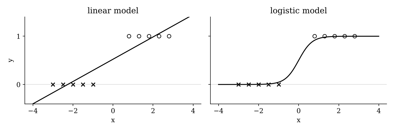
Example. Suppose each input has a single feature. Points with label \(y = 0\) sit on the left of the line, and points with label \(y = 1\) on the right. To use regression, we first plot the labels against the inputs, so there is something to fit.
Fitting a straight line (left) does not capture the relationship well; the data are not really linear. A much better model (right) is the logistic function \[ f(x) := \frac{1}{1 + e^{-w \cdot x}}. \] Its S shape describes how the label switches from 0 to 1 far better than a line or polynomial can.
This leaves three questions:
Logistic regression comes from probability and statistics, so we answer the first question with a probabilistic model.
Recall the probabilistic interpretation of OLS from Chapter 1.2. We modeled each label as \[ Y_i \sim \mathcal{N}(f(x_i), 1), \qquad \text{where } f(x) := w \cdot x \text{ for some } w \in \mathbb{R}^{d+1}. \] The mean of the label is a linear function of the input.
For classification, labels are 0 or 1, so a normal distribution no longer makes sense. The natural distribution for a random variable that is either 0 or 1 is the Bernoulli: \[ Y_i \sim \text{Bernoulli}(f(x_i)). \] The parameter of a Bernoulli random variable is its probability of success. Here, \(f(x_i)\) is the probability that \(x_i\) has label 1. It depends on the input: if we are labeling whether an image shows a cat, \(f(x_i)\) should be close to 1 for a picture of a cat and close to 0 for a picture of a classroom.
First idea: model \(f(x)\) as linear, \(f(x) := w \cdot x\), just like OLS. No! We need \(f(x) \in (0, 1)\), because it is a probability. A linear function can output any real number, which would not give a valid distribution.
So instead, look for a transformation of the probability that lives in \(\mathbb{R}\), and model that with a linear function.
Attempt 1: the odds. The ratio of the probability of success to the probability of failure, \[ \text{odds}(f(x)) := \frac{f(x)}{1 - f(x)} \in (0, \infty). \] Look at the extremes. As \(f(x) \to 0\), the odds approach 0. As \(f(x) \to 1\), the denominator shrinks and the odds grow without bound. Progress, but the odds are never negative, so a linear model still doesn’t fit.
Attempt 2: the log-odds, or logit. \[ \text{logit}(f(x)) := \log \frac{f(x)}{1 - f(x)} \in \mathbb{R}. \] The log maps \((0, \infty)\) onto all of \(\mathbb{R}\), negative values included. This is a quantity a linear model can reasonably describe.
Assume \(\log \dfrac{f(x)}{1 - f(x)} := w \cdot x\) for some \(w \in \mathbb{R}^{d+1}\), and solve for \(f(x)\): \[ \begin{aligned} &\frac{f(x)}{1 - f(x)} = e^{w \cdot x} \\ \iff\;& f(x) = e^{w \cdot x}\big(1 - f(x)\big) = e^{w \cdot x} - e^{w \cdot x} f(x) \\ \iff\;& \big(1 + e^{w \cdot x}\big) f(x) = e^{w \cdot x} \\ \iff\;& f(x) = \frac{e^{w \cdot x}}{1 + e^{w \cdot x}} = \frac{1}{1 + e^{-w \cdot x}}. \end{aligned} \] That is exactly the logistic function. Logistic regression models the log-odds of the label with a linear function, and that assumption forces \(f\) to be logistic. You can now derive the logistic function from scratch. The probabilistic model also tells us how to define a loss.
Setup (logistic regression)
Here \(p(y_i)\) is an actual probability, since \(Y_i\) is discrete. Because \(Y_i \sim \text{Bernoulli}(f(x_i))\), \[ \begin{cases} y_i = 1 \;\Rightarrow\; p(y_i) = f(x_i), \\ y_i = 0 \;\Rightarrow\; p(y_i) = 1 - f(x_i). \end{cases} \] To combine the two cases into a single formula, \[ p(y_i) = f(x_i)^{y_i} \big(1 - f(x_i)\big)^{1 - y_i}. \] When \(y_i = 1\), only the first factor survives; when \(y_i = 0\), only the second.
As in Chapter 1.2, maximizing the likelihood is the same as maximizing the log-likelihood, which turns the product into a sum: \[ \log \mathcal{L}(w) = \sum_{i=1}^n \log p(y_i) = \sum_{i=1}^n \Big( y_i \log f(x_i) + (1 - y_i) \log\big(1 - f(x_i)\big) \Big), \quad \text{where } f(x_i) = \frac{1}{1 + e^{-w \cdot x_i}}. \]
This looks complicated, but it is just a function of \(w\). Given the data and any candidate \(w\), you can compute it, and we want the \(w\) that makes it as large as possible. Equivalently, we minimize the loss \[ L(w) := -\log \mathcal{L}(w). \]
Once we have \(w\), \(f(x)\) gives the probability that \(x\) has label 1. To output a discrete label, threshold it: \[ \mathbb{1}\{f(x) > \tfrac12\} := \begin{cases} 1 & \text{if } \dfrac{1}{1 + e^{-w \cdot x}} > \tfrac12, \\[4pt] 0 & \text{otherwise.} \end{cases} \]
There is nothing special about \(\tfrac12\). The threshold is a tunable hyperparameter. Depending on the problem, a different threshold may be more appropriate, and you can choose it with cross-validation or a train/validation/test split. You will do this in Homework 2.1.
Algorithm (gradient descent). Given a differentiable loss function \(L(\theta)\):
Finding a good \(\theta\) is hard, but finding some \(\theta\) is easy, so we start anywhere (all zeros is fine) and keep improving it. The scalar \(\eta > 0\) is the step size, also called the learning rate. Each step subtracts a scaled version of the gradient, which is where the name comes from. Gradient descent is also how deep neural networks are trained, so it will come up again.
Remark. With an “appropriate” \(\eta\), if \(L\) is convex, gradient descent converges to a global minimizer.
Run gradient descent to find \(\operatorname*{argmin}_x L(x)\) for \(L(x) = x^2\), with \(\eta = 0.1\). Of course the answer is \(x = 0\); let’s check that gradient descent finds it.
Observation. \(x^{(t)}\) moves “downhill” toward the global minimum at \(x = 0\). Each step is smaller than the last, because the gradient shrinks as we approach the minimum. At \(x = 0\), the gradient is exactly zero, so we have found a stationary point and can stop.
Work through this example yourself. Numeric problems like it can appear on the module assessment.
Recall the loss \[ L(w) := -\log \mathcal{L}(w) = -\sum_{i=1}^n \Big( y_i \log f(x_i) + (1 - y_i) \log\big(1 - f(x_i)\big) \Big), \qquad f(x_i) = \frac{1}{1 + e^{-w \cdot x_i}}. \] Its gradient is \[ \nabla L(w) = \sum_{i=1}^n \big( f(x_i) - y_i \big)\, x_i. \] The derivation is a calculus exercise. More interesting is what it says: \[ \text{update direction} = \sum_i \big(\text{predicted probability} - \text{label}\big)\, x_i, \] and the update is \(w^{(t+1)} \leftarrow w^{(t)} - \eta\, \nabla L(w^{(t)})\).
Why is moving toward \(x_i\) the right thing to do? Moving \(w\) toward \(x_i\) makes \(w \cdot x_i\) larger, so \(-w \cdot x_i\) is smaller, so \(e^{-w \cdot x_i}\) is smaller, so \(f(x_i) = \frac{1}{1 + e^{-w \cdot x_i}}\) is larger. The model becomes more confident that \(x_i\) has label 1, which is exactly what we wanted.
In general, each step looks at the points the model gets wrong, and moves \(w\) toward or away from each one depending on how far off its prediction is. This idea comes back in Chapters 2.5 and 2.7.