Last time: Naive Bayes. We approximated the Bayes classifier by \[ \begin{aligned} \hat f(x) &:= \operatorname*{argmax}_{y \in \mathcal{Y}} p(y \mid x) \\ &= \operatorname*{argmax}_{y \in \mathcal{Y}} p(y)\, p(x \mid y) \\ &= \operatorname*{argmax}_{y \in \mathcal{Y}} p(y) \prod_{j=1}^d p(x^{(j)} \mid y), \qquad \text{features independent.} \end{aligned} \]
Naive Bayes has two weaknesses. First, the features are often not independent in real data. Second, even when they are, a feature’s distribution may not look like any familiar parameterized distribution, so estimating it well can be hard.
That motivates a different perspective. Instead of learning a global distribution over inputs and labels, look only at what happens locally.
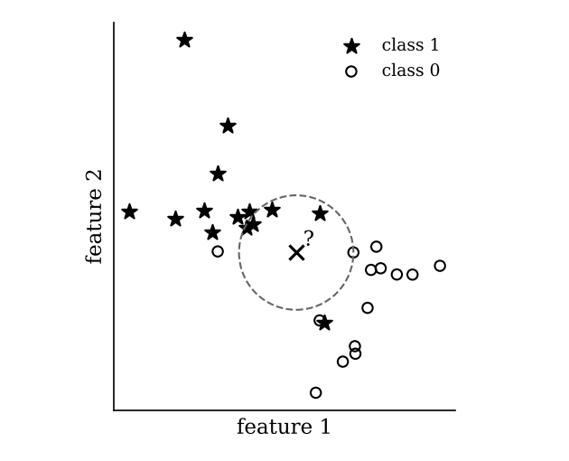
To classify a new point (the ×), look at the geometry of the labeled data around it. The dashed circle contains its 5 nearest neighbors.
Setup (k-nearest neighbors)
The algorithm is described by its name. To classify \(x\), compute its distance to every training point, find the \(k\) closest, and take the majority vote of their labels.
If \(n, k \to \infty\) and \(k/n \to 0\), then the kNN classifier converges to the Bayes classifier.
With enough data, and a neighborhood that grows, but more slowly than the data, kNN is as good as it gets. Compare the consistency result for kernel regression in Chapter 1.4.
To use kNN, we need to say what nearest means. There are many ways to measure “closeness” between \(x_1, x_2 \in \mathcal{X}\):
Examples.
kNN relies on a locality assumption: that the notion of a “neighbor” is meaningful. That seems far more reasonable than Naive Bayes’ independence assumption, and in 2D or 3D it clearly holds. But our geometric intuition comes from two and three dimensions, and it does not carry over to high dimensions. In high dimensions, the notion of a neighbor breaks down.
Let \(X, X' \sim \mathcal{N}(0, I_d)\) independently. Then for all \(\varepsilon > 0\), \[ \mathbb{P}\left( \left| \frac{\|X - X'\|^2}{2d} - 1 \right| \geq \varepsilon \right) \leq \frac{2}{\varepsilon^2 d}. \]
This is one of a whole family of results of the same flavor, which is why it is called concentration of measure.
Proof. Notice that \(X - X' \sim \mathcal{N}(0, 2I_d)\). The difference of independent Gaussians is Gaussian: the means subtract, giving \(0\), and the variances add, giving \(1 + 1 = 2\) in each coordinate. Intuitively, subtracting two random quantities combines the randomness of both. Writing each coordinate of \(X - X'\) as \(\sqrt{2}\) times a standard normal, \[ \|X - X'\|^2 \sim 2\chi^2(d) \quad\Rightarrow\quad \mathbb{E}\big[\|X - X'\|^2\big] = 2d, \qquad \text{Var}\big(\|X - X'\|^2\big) = 2^2 \cdot (2d) = 8d. \] (Scaling a random variable by \(2\) scales its variance by \(2^2\).)
Consider \(Z := \dfrac{\|X - X'\|^2}{2d}\). Then \[ \mathbb{E}[Z] = 1, \qquad \text{Var}(Z) = \frac{8d}{(2d)^2} = \frac{2}{d}. \] By Chebyshev’s inequality, \[ \mathbb{P}\big(|Z - 1| \geq \varepsilon\big) \leq \frac{\text{Var}(Z)}{\varepsilon^2} = \frac{2}{\varepsilon^2 d} \qquad \text{for all } \varepsilon > 0. \qquad \blacksquare \]
Remark. As \(d \to \infty\), \[ \mathbb{P}\left( \left| \frac{\|X - X'\|^2}{2d} - 1 \right| \geq \varepsilon \right) \to 0, \] however small \(\varepsilon\) is. So:
If you sample random points in high dimensions, almost every pair is about \(\sqrt{2d}\) apart. Your \(k\) nearest neighbors are then barely closer than your \(k\) farthest. Similar results hold for cosine similarity and \(\ell_p\) norms in general: most predefined distances behave poorly when data have many features.
We sample 600 points from \(\mathcal{N}(0, I_d)\) and plot a histogram of all pairwise Euclidean distances, for increasing \(d\). The dashed line marks \(\sqrt{2d}\).
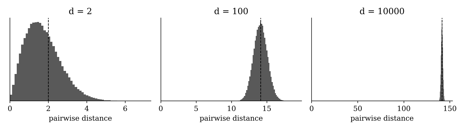
In 2 dimensions, the distances cover a wide range. By \(d = 10{,}000\), almost every pair is about \(\sqrt{20{,}000} \approx 141\) apart. Try other values of \(d\) yourself.
If predefined distances fail in high dimensions, learn a notion of distance from the data!
Task (metric learning)
Classical metric learning learns a transformation of the Euclidean distance with these properties, but in practice those methods have not worked well. The modern approach is to learn an embedding function \[ \phi : \mathcal{X} \to \mathbb{R}^d \] with a neural network, so that a simple predefined distance, such as cosine similarity, becomes meaningful after embedding. If you have heard of contrastive learning, that is exactly this idea. The model is trained on pairs labeled “similar” or “dissimilar.” The contrastive loss pulls the embeddings of similar pairs together and pushes dissimilar pairs apart. You will be able to understand how these models work after the deep learning module.
Suppose we have a small collection of documents about machine learning concepts:
documents = [
    "Gradient descent updates parameters using the derivative of the loss.",
    "We use MLE to estimate model parameter from sample data.",
    "The model was deployed to production using a cloud service.",
    "Regularization reduces overfitting by penalizing large model weights.",
    "Metric learning is a ML technique that automatically learns to measure similarity",  # target
]
query = "We need a method to learn distance from data."
A human would say the last document is the most relevant to the query. Can a computer find it?
Attempt 1: TF-IDF vectors and cosine similarity. TF-IDF is a standard way to turn text into vectors. Ranking the documents by cosine similarity to the query gives:
0.335 - We use MLE to estimate model parameter from sample data.
0.052 - The model was deployed to production using a cloud service.
0.043 - Metric learning is a ML technique that automatically learns to measure similarity
0.0   - ...
The MLE sentence wins, mostly because it shares words like “data” with the query. Cosine similarity in this vector space is not a great notion of closeness.
Attempt 2: a learned embedding. Using a pretrained sentence embedding model (all-MiniLM-L6-v2), trained with a contrastive loss, and then the same cosine similarity:
0.618 - Metric learning is a ML technique that automatically learns to measure similarity
0.358 - We use MLE to estimate model parameter from sample data.
0.232 - Regularization reduces overfitting by penalizing large model weights.
0.204 - Gradient descent updates parameters using the derivative of the loss.
Now the target document ranks first. The distance didn’t change; the representation did.