Last time we saw that the kNN classifier converges to the optimal Bayes classifier. A naive implementation of kNN has two practical problems:
Take \(\mathcal{X} = \mathbb{R}\) first. A better way to find the neighbor of a test point \(x_t\) among \(x_1, \dots, x_n\) is binary search. Split the line at the median, recursively split each half at its median, and search down the resulting tree. This improves the search time to \(O(\log n)\).
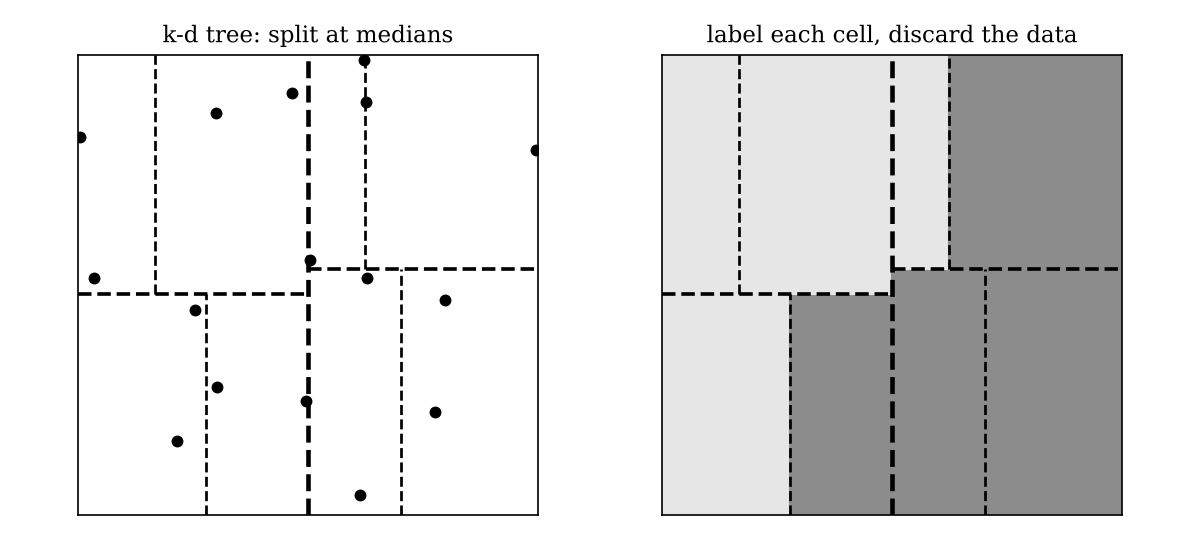
For \(\mathcal{X} = \mathbb{R}^d\), the analogous data structure is a \(k\)-d tree. It partitions the input space into disjoint cells: split at the median of one feature, then recursively split each half at the median of another feature, cycling through the features. With a \(k\)-d tree, the search time becomes \(O(d \log n)\).
The \(k\)-d tree helps with space too. Instead of keeping all the training data around at test time, label each cell with the majority label of its training points, then discard the data. All we need to remember is how the space is partitioned and the label of each cell.
Notice that building a \(k\)-d tree does not use the labels. It splits at medians, so it is not optimizing for classification accuracy at all.
The idea of decision tree classifiers is to keep the partitioning, but choose the splits more carefully. Rather than picking an arbitrary feature and splitting at its median, we should select the feature and threshold that reduce label uncertainty.
A decision tree is usually drawn, as the name suggests, as a tree. The root is the whole input space. Each internal node splits its cell on one feature, and the leaves are the final cells. We keep splitting until each cell is (mostly) pure: all, or nearly all, of its training points share one label. A pure cell is easy to label.
This chapter covers how to construct a decision tree and make predictions with it, and how to improve its performance with bagging.
For clarity, we focus on binary features. Extending to non-binary discrete or continuous features follows the same principle.
A decision tree is constructed by recursively partitioning the input space into disjoint cells. Like any recursion, we need a recursive step (how to split a cell into smaller ones) and a base case (when to stop).
Recursive step. At each node, with current cell \(C\), select the feature \(F\) that minimizes the weighted impurity after splitting: \[ \operatorname*{argmin}_F \Big[\, p_1 \cdot u(C_{F=1}) + p_0 \cdot u(C_{F=0}) \,\Big], \] where
Then recurse on \(C_{F=1}\) and \(C_{F=0}\).
Common choices of \(u(\cdot)\). Write \(p_y\) for the fraction of points in cell \(C\) with label \(y\).
Stopping criteria. When to stop splitting is a design choice. Common criteria, often combined:
min_samples_split
samples. Splitting tiny cells produces noisy leaves.max_depth is reached. Deeper trees
make less stable predictions, so limiting depth helps the model
generalize.Given a new input \(x\):
If you stop growing the tree before every leaf is pure, the leaves contain a mix of labels, which is why we take the majority.
Let’s build the root split for a binary spam classifier (\(y = 1\) means spam). We have 8 training emails and the two binary features from Chapter 2.2:
F_free: does the email contain the word “free”?F_win: does it contain “win”?F_free |
F_win |
\(y\) | |
|---|---|---|---|
| 1 | 1 | 1 | 1 |
| 2 | 1 | 1 | 1 |
| 3 | 1 | 0 | 1 |
| 4 | 1 | 0 | 0 |
| 5 | 0 | 1 | 1 |
| 6 | 0 | 0 | 0 |
| 7 | 0 | 1 | 0 |
| 8 | 0 | 1 | 0 |
We use classification error as the impurity measure.
Step 1: root impurity. Four of the eight emails are spam, so \(p_1 = p_0 = \tfrac12\) and \[ u(C) = 1 - \max\big(\tfrac12, \tfrac12\big) = 0.5. \]
Step 2: choose the root split. Compute the weighted impurity after splitting on each feature.
F_free. \(C_{F=1}\) is emails 1–4, with labels \(1, 1, 1, 0\), so \(u = 1 - \tfrac34 = \tfrac14\). \(C_{F=0}\) is emails 5–8, with labels \(1, 0, 0, 0\), so \(u = \tfrac14\). The weighted impurity is
\[
\tfrac48 \cdot \tfrac14 + \tfrac48 \cdot \tfrac14 = 0.25.
\]F_win. \(C_{F=1}\) is emails 1, 2, 5, 7, 8, with
labels \(1, 1, 1, 0, 0\), so \(u = 1 - \tfrac35 = \tfrac25\). \(C_{F=0}\) is emails 3, 4, 6, with labels
\(1, 0, 0\), so \(u = \tfrac13\). The weighted impurity is
\[
\tfrac58 \cdot \tfrac25 + \tfrac38 \cdot \tfrac13 = 0.25 + 0.125 =
0.375.
\]Which feature should you split on?
F_free, because it gives the lower weighted impurity,
\(0.25 < 0.375\). Both splits reduce
impurity from the root’s \(0.5\), but
F_free reduces it more. After the split, each cell is 75%
one label.
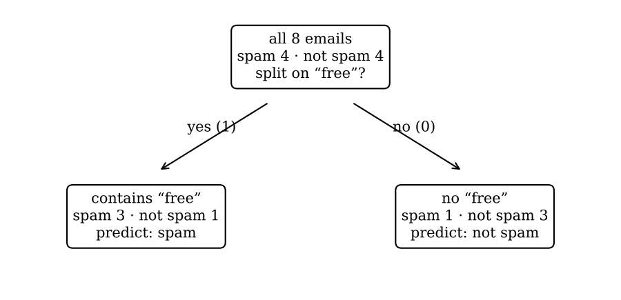
What happens next? Recursion. We have split the dataset into two cells, \(C_L = \{x : x_F = 1\}\) and \(C_R = \{x : x_F = 0\}\). To grow the tree, repeat the same procedure on each cell: compute its impurity, choose the best split within it, and partition it into sub-cells. The stopping criteria decide when to stop. With only 8 examples, we would probably stop here.
Let’s train a decision tree on a real dataset: the Spambase email dataset from Homework 2.1, with an 80/20 train/test split and no hyperparameter tuning.
from sklearn.tree import DecisionTreeClassifier
deep_tree = DecisionTreeClassifier(random_state=4721).fit(X_train, y_train)
Training accuracy: 0.9995
Test accuracy: 0.9012What do you notice? The model classifies the training data almost perfectly, but there is a sizeable gap to the test accuracy: it overfits. This is typical of decision trees. Without a depth limit they are extremely flexible: you can always keep splitting until every leaf holds a single training point, and then the training data are classified perfectly. You could restrict the depth or tune hyperparameters, but in practice people use bagging.
Idea (bagging): train many models on slightly different datasets, e.g. bootstrap samples, then vote their predictions.
Bagging is a general ensemble strategy that works with any high-variance model, though it is especially effective with decision trees. We rarely have many independent datasets, so we create slightly different ones by bootstrap sampling: drawing samples from our one dataset with replacement. In terms of the bias–variance tradeoff, bagging keeps the bias roughly the same, since each model comes from the same model class, but reduces the variance by averaging the predictions of many models.
For decision trees, combining bagging with random feature selection gives the random forest:
max_features).The random feature selection makes the trees even more different from one another, which makes averaging more effective. To predict, each tree votes, and the forest outputs the majority.
from sklearn.ensemble import RandomForestClassifier
rf = RandomForestClassifier(n_estimators=300, random_state=4721).fit(X_train, y_train)
Deep tree | train acc = 0.9995 | test acc = 0.9012
RandomForest | train acc = 0.9995 | test acc = 0.9511The training accuracy is still near perfect, but the test accuracy improves significantly.