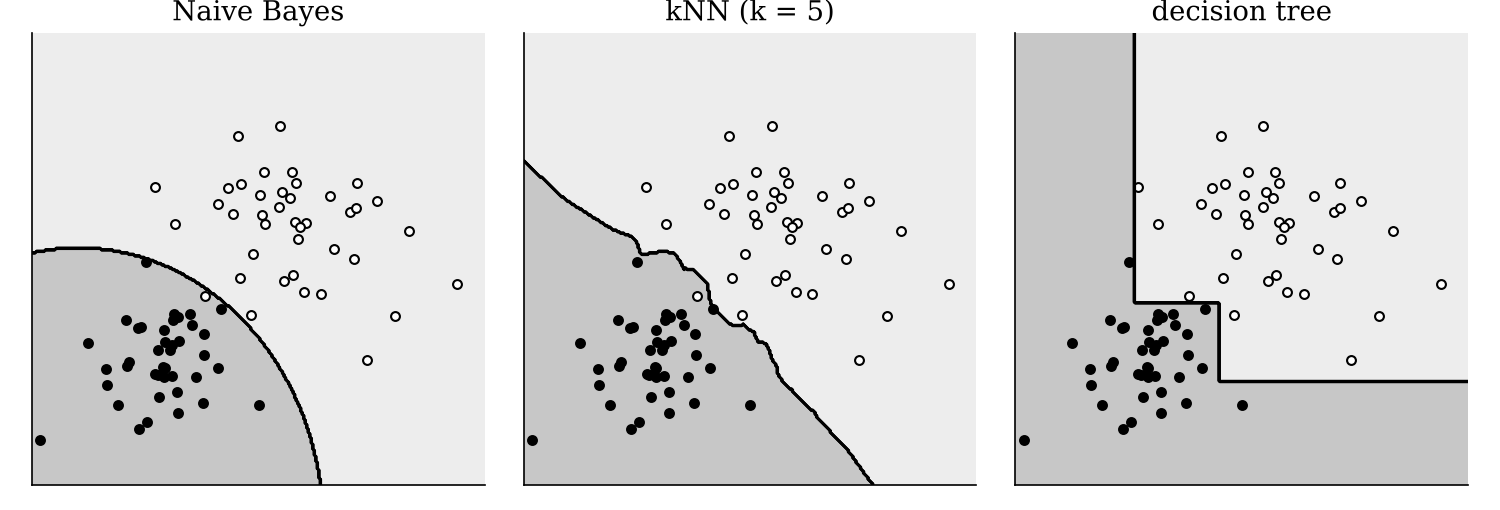
Let’s look at how the classifiers we have seen so far carve up the input space.
Observation: knowing the boundary is enough for classification! For each of these classifiers, the boundary is only implicit in the learned model.
Idea. Learn the decision boundary directly, starting with the simplest shape a boundary can have. Assume the data can be separated by a linear decision boundary. Such data are called linearly separable. We again focus on binary classification; extending to more classes is a good exercise.
As usual, after bias lifting the bias is absorbed into the weights. If the data are linearly separable, there is a \(w \in \mathbb{R}^{d+1}\) such that \[ \begin{cases} y_i = +1 \iff w \cdot x_i > 0, \\ y_i = -1 \iff w \cdot x_i < 0. \end{cases} \] So the goal is: find \(w \in \mathbb{R}^{d+1}\) such that \(\text{sign}(w \cdot x_i) = y_i\) for all \(i\).
Setup (perceptron)
Both compute a linear score \(w \cdot x\). Logistic regression turns the score into a probability with the sigmoid; the perceptron turns it into a discrete label with the sign function. You can think of the perceptron as a discrete cousin of logistic regression. Like logistic regression, and unlike kNN, after training we only need to store the \(d + 1\) numbers in \(w\).
Algorithm (learning perceptron weights). Given data with bias included, \(S := \{(x_1, y_1), \dots, (x_n, y_n)\} \subset \mathbb{R}^{d+1} \times \{+1, -1\}\):
Terminate when no such training sample exists.
As with gradient descent, finding the best weights is hard, but finding some weights is easy, so we start at zero and improve. Each step finds a mistake and corrects for it:
(Compare the gradient update for logistic regression in Chapter 2.1, which also moves toward or away from misclassified points.) If \(w \cdot x = 0\), the point lies exactly on the boundary; we count that as a mistake, so it triggers an update.
Remarks.
Assume the training data are linearly separable with margin \(\gamma\). Let \(R = \max_{x \in S} \|x\|\). Then the perceptron terminates in at most \[ T := \Big(\frac{R}{\gamma}\Big)^2 \text{ rounds.} \]
So the converse also holds: when the data are separable, the perceptron finds a separating hyperplane, and we have a bound on how long it takes. Data that are well separated relative to their spread, so that \(R/\gamma\) is small, are learned quickly. We state this without proof.
The XOR function outputs 1 exactly when its two binary inputs differ. To train a perceptron, first lift the bias (append a 1 to each input) and relabel the outputs as \(\pm 1\):
| \(x\) | input | XOR | \(y\) |
|---|---|---|---|
| \((0, 0, 1)\) | \((0, 0)\) | 0 | \(-1\) |
| \((0, 1, 1)\) | \((0, 1)\) | 1 | \(+1\) |
| \((1, 0, 1)\) | \((1, 0)\) | 1 | \(+1\) |
| \((1, 1, 1)\) | \((1, 1)\) | 0 | \(-1\) |
Initialize \(w^{(0)} = (0, 0, 0)\), and take the data in the order above.
| \(t\) | \(x\) | \(y\) | \(w^{(t-1)} \cdot x\) | \(w^{(t)}\) |
|---|---|---|---|---|
| 1 | \((0, 0, 1)\) | \(-1\) | \(0\) | \((0, 0, -1)\) |
| 2 | \((0, 1, 1)\) | \(+1\) | \(-1\) | \((0, 1, 0)\) |
| 3 | \((1, 0, 1)\) | \(+1\) | \(0\) | \((1, 1, 1)\) |
| 4 | \((1, 1, 1)\) | \(-1\) | \(3\) | \((0, 0, 0)\) |
Every step is a mistake. After four updates we are back where we started, at \(w = (0, 0, 0)\), so the algorithm will not terminate.
The reason: plot the four inputs, and the two \(+1\) points sit on one diagonal of the unit square while the two \(-1\) points sit on the other. No straight line separates them, so XOR is not linearly separable. The perceptron is too weak to learn even this tiny function.
We generate a small, linearly separable 2D dataset and train the perceptron four times. The training data are the same each time, but each run starts at a different point in the data (index 0, 10, 30 or 70) and cycles through from there.
def perceptron_cyclic_start(X, y, start_idx=0, max_epochs=500):
    Xb = np.hstack([X, np.ones((X.shape[0], 1))])          # bias lifting
    w = np.zeros(Xb.shape[1])
    order = np.roll(np.arange(len(X)), -start_idx)
    for _ in range(max_epochs):
        mistakes = 0
        for i in order:
            if y[i] * (w @ Xb[i]) <= 0:                     # mistake (or on the boundary)
                w = w + y[i] * Xb[i]
                mistakes += 1
        if mistakes == 0:
            return w
    return w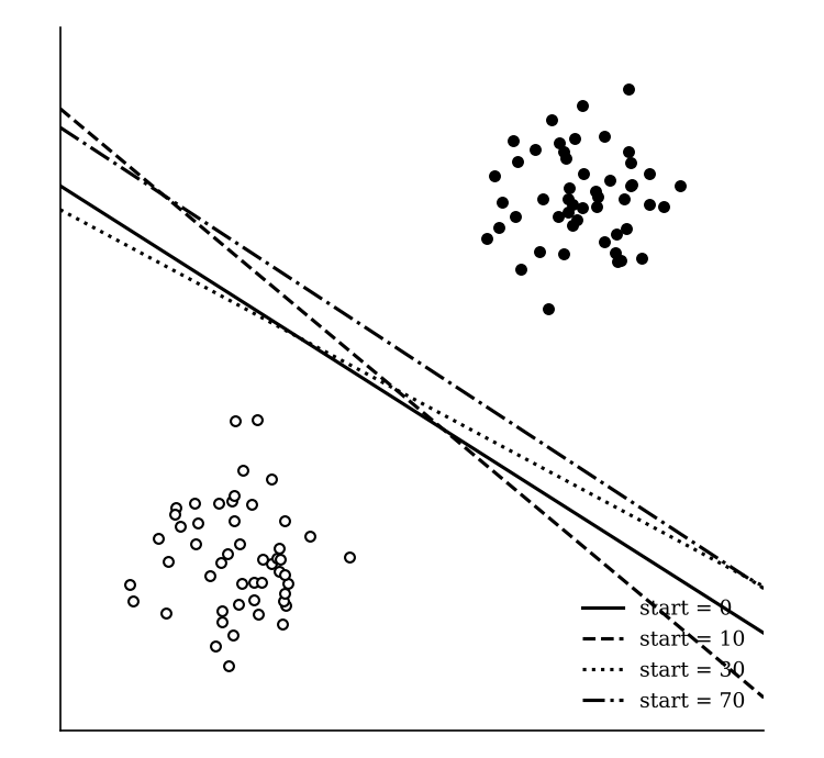
Each run finds a hyperplane that separates the data perfectly, but each run finds a different one.
How can we make the perceptron more expressive? Start by visualizing it. Without bias lifting, the perceptron maps \[ x \in \mathbb{R}^d \;\xrightarrow{\;w,\, b\;}\; w \cdot x + b \in \mathbb{R} \;\xrightarrow{\;\text{sign}\;}\; \text{sign}(w \cdot x + b), \] which we can draw compactly as \(x \xrightarrow{w, b}\) (unit).
Idea. Use many units. Apply \(m\) different sets of weights and biases \((w_1, b_1), \dots, (w_m, b_m)\) to the same input, getting \(m\) numbers, then combine them into one output.
Stacking the weight vectors as the rows of a matrix \(W \in \mathbb{R}^{m \times d}\) and the biases into a vector \(b \in \mathbb{R}^m\): \[ x \in \mathbb{R}^d \;\xrightarrow{\;W,\, b\;}\; Wx + b \in \mathbb{R}^m \;\xrightarrow{\text{element-wise activation}}\; \phi(Wx + b) \in \mathbb{R}^m \;\longrightarrow\; \text{output}. \] Instead of the sign function, we allow any nonlinear activation function \(\phi\), applied to each entry separately. To combine the \(m\) hidden values into one output, the simplest choice is a linear function.
Model (MLP with one hidden layer)
Remark (universal approximation theorem). For suitable \(\phi\), an MLP with one hidden layer can approximate a very broad class of functions. Precisely, if you have taken real analysis: continuous functions on a compact domain. XOR is in that class, so adding a hidden layer fixes the problem above.
A few notes:
Summary.
Next time: support vector machines, which fix all three problems by looking for the hyperplane with the largest margin.