Last time: the perceptron. We learned \[ \hat f(x) = \text{sign}(w^\top x + b) \quad \text{for } w \in \mathbb{R}^d,\ b \in \mathbb{R}, \qquad \text{such that } y_i(w^\top x_i + b) > 0 \;\; \forall i. \] (This chapter keeps the bias \(b\) separate rather than lifting it, for a reason we will see shortly.)
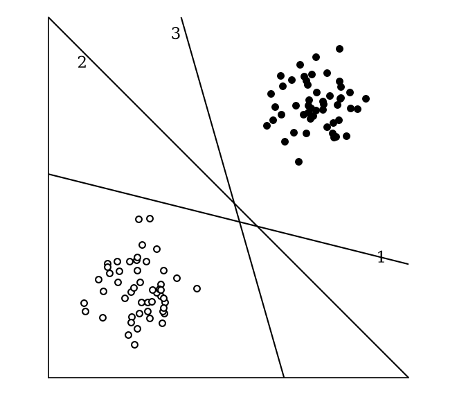
If the data are linearly separable, many hyperplanes separate them. Which one would you choose? Most people pick the one in the middle. If there is any noise or uncertainty in new data, a boundary that stays far from both classes leaves more room for error before it starts making mistakes. The perceptron can return any of these lines.
Today: learn the linear decision boundary with the maximum margin. That is easy to say in words; writing it down as an optimization problem takes some work, and rewriting that problem in a second form tells us where the name “support vectors” comes from.
Recall. Given \(x_i \in \mathbb{R}^d\) and a hyperplane \(g(x) = w \cdot x + b = 0\), the distance from \(x_i\) to the hyperplane is \[ \frac{|w \cdot x_i + b|}{\|w\|}. \] If this is unfamiliar, it is worth reviewing in your linear algebra notes.
Definition. Given data \((x_1, y_1), \dots, (x_n, y_n) \in \mathbb{R}^d \times \{+1, -1\}\) that are linearly separable, and a hyperplane \(g(x) = w \cdot x + b = 0\) that correctly classifies the data, the margin is \[ \gamma(w, b) := \min_i \frac{y_i(w \cdot x_i + b)}{\|w\|} = \frac{\min_i y_i(w \cdot x_i + b)}{\|w\|}. \] The margin is the distance from the hyperplane to the closest training point. Because the hyperplane classifies every point correctly, \(y_i(w \cdot x_i + b) = |w \cdot x_i + b|\), so multiplying by the label removes the absolute value.
Idea. The objective is \[ \max_{w, b} \gamma(w, b) \quad \text{such that } y_i(w^\top x_i + b) > 0 \;\; \forall i. \] This states our goal exactly, but a maximization of something defined by a minimization is hard to work with or interpret. Let’s simplify.
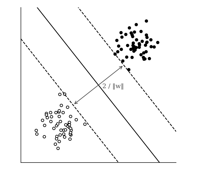
Geometrically, the boundary \(w \cdot x + b = 0\) sits between two parallel lines, \(w \cdot x + b = +1\) and \(w \cdot x + b = -1\). All the \(+1\) points lie on or beyond the first, and all the \(-1\) points on or beyond the second. The gap between the dashed lines is \(2/\|w\|\), twice the margin. The SVM pushes these lines as far apart as possible. “Hard margin” means we require every point to be correctly classified, so the data must be linearly separable.
Then no \((w, b)\) satisfies all the constraints. Idea: introduce slack variables \(\varepsilon_1, \dots, \varepsilon_n\) to allow misclassified points. Each constraint is relaxed to \(y_i(w^\top x_i + b) \geq 1 - \varepsilon_i\), so point \(i\) may sit inside the margin, or even on the wrong side, by an amount \(\varepsilon_i\). We don’t want to hand out too much slack, so we also penalize the total slack in the objective: \[ \boxed{\; \min_{w, b, \varepsilon} \tfrac12 \|w\|^2 + C \sum_{i=1}^n \varepsilon_i \quad\text{such that}\quad y_i(w^\top x_i + b) \geq 1 - \varepsilon_i, \;\; \varepsilon_i \geq 0. \;} \] This is what people usually mean by “the” support vector machine.
Setup (support vector machines)
Question: why is it called a support vector machine, and not, say, a “maximum margin machine”? To answer this, we rewrite the optimization problem in a different form.
Definition. Given a constrained optimization problem \[ \begin{aligned} \text{minimize}_\theta \quad & f(\theta) \\ \text{such that} \quad & g_i(\theta) \leq 0 \quad \text{for } 1 \leq i \leq n, \end{aligned} \] the Lagrange function is defined as \[ \mathcal{L}(\theta, \lambda) := f(\theta) + \sum_{i=1}^n \lambda_i g_i(\theta), \] where \(\lambda_i \geq 0\) are new variables, one per constraint, called dual variables. The definition may look strange at first; the observations below explain it.
Example (the Lagrange function for the hard-margin SVM). Rewriting each constraint as \(1 - y_i(w \cdot x_i + b) \leq 0\), and calling the dual variables \(\alpha_i\): \[ \mathcal{L}(w, b, \alpha) := \tfrac12 \|w\|^2 + \sum_{i=1}^n \alpha_i \big(1 - y_i(w \cdot x_i + b)\big). \]
Observation. For any feasible \(\theta\) (one that satisfies all the constraints) and all \(\lambda_i \geq 0\), we have \(\mathcal{L}(\theta, \lambda) \leq f(\theta)\), because every added term \(\lambda_i g_i(\theta)\) is \(\leq 0\). Taking the max over \(\lambda\):
So the optimal value of the original constrained problem is \[ p^* = \min_\theta \max_{\lambda_i \geq 0} \mathcal{L}(\theta, \lambda), \] called the primal. Infeasible \(\theta\) get value \(\infty\), so the outer minimization automatically avoids them. The constraints are now built into the objective. That alone doesn’t make the problem easier to interpret, but it sets up the next step.
Let \[ d^* = \max_{\lambda_i \geq 0} \underbrace{\min_\theta \mathcal{L}(\theta, \lambda)}_{\text{unconstrained in } \theta}. \] For the SVM optimization problem, we have \(d^* = p^*\). Further, there exist optimal solutions \(\theta^*, \lambda^*\) such that \[ \mathcal{L}(\theta^*, \lambda^*) = d^* = p^*. \]
The dual \(d^*\) swaps the order of the min and the max. In general you cannot do that, but for the SVM you can. The payoff is that, for fixed \(\lambda\), the inner minimization over \(\theta\) has no constraints, so we can solve it by setting derivatives to zero, and express the original variables in terms of the dual variables.
Lagrangian: \(\mathcal{L}(w, b, \alpha) = \tfrac12 \|w\|^2 + \sum_{i=1}^n \alpha_i \big(1 - y_i(w \cdot x_i + b)\big)\).
Primal: \(p^* = \min_{w, b} \max_{\alpha \geq 0} \mathcal{L}(w, b, \alpha)\).
Dual: \(d^* = \max_{\alpha \geq 0} \min_{w, b} \mathcal{L}(w, b, \alpha)\). The inner problem is unconstrained, so we can solve for the optimal \(w\) and \(b\) in terms of \(\alpha\): \[ \begin{aligned} \frac{\partial}{\partial w} \mathcal{L}(w, b, \alpha) &= w - \sum_{i=1}^n \alpha_i y_i x_i = 0 &&\Rightarrow\quad w = \sum_{i=1}^n \alpha_i y_i x_i, \\ \frac{\partial}{\partial b} \mathcal{L}(w, b, \alpha) &= -\sum_{i=1}^n \alpha_i y_i = 0 &&\Rightarrow\quad \sum_{i=1}^n \alpha_i y_i = 0. \end{aligned} \] Plugging these back into \(\mathcal{L}\) (a good exercise; several terms cancel), \[ \min_{w, b} \mathcal{L}(w, b, \alpha) = \sum_{i=1}^n \alpha_i - \frac12 \sum_{i, j} \alpha_i \alpha_j y_i y_j (x_i \cdot x_j). \]
Hard-margin SVM, dual form: \[ \max_\alpha \; \sum_{i=1}^n \alpha_i - \frac12 \sum_{i, j} \alpha_i \alpha_j y_i y_j (x_i \cdot x_j) \quad \text{such that } \sum_{i=1}^n \alpha_i y_i = 0, \quad \alpha_i \geq 0. \]
In Homework 2.2 you will carry out this derivation for the soft-margin SVM, with slack variables.
Remarks.
A point with \(\alpha_i^* \neq 0\) must lie on the margin. The converse does not always hold: occasionally a point lies exactly on the margin but has \(\alpha_i^* = 0\). In typical data, the support vectors and the points on the margin coincide.
We use the same toy dataset as the perceptron demo, and solve the SVM dual with scikit-learn. A very large \(C\) approximates the hard-margin SVM.
from sklearn.svm import SVC

clf = SVC(kernel="linear", C=1e6)       # large C ~ hard margin
clf.fit(X, y)

dual_coef = clf.dual_coef_.ravel()      # alpha_i * y_i, for support vectors only
SV = clf.support_vectors_               # the support vectors
w = (dual_coef[:, None] * SV).sum(axis=0)   # w* = sum_i alpha_i y_i x_i
b = clf.intercept_[0]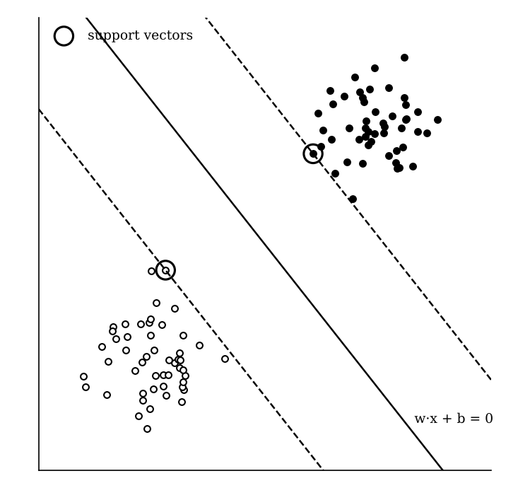
Out of 100 training points, only two have a non-zero \(\alpha_i\). Circled above, they are exactly the points touching the margin lines \(w^* \cdot x + b^* = \pm 1\), and \(w^*\) is computed from them alone. Unlike the perceptron, the SVM’s answer does not depend on the order of the data: the maximum-margin hyperplane is unique.
Next time: the dual form has one more gift. Notice that the data appear in the dual only through dot products \(x_i \cdot x_j\). That observation lets us learn nonlinear decision boundaries.