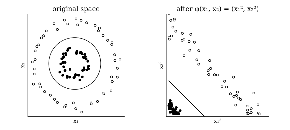
So far in this module, we have learned linear decision boundaries: the perceptron returns a separating hyperplane, and the SVM returns the one with the maximum margin. What decision boundary separates the following data?
No straight line works on the left. But an ellipse does. We can parameterize one as \[ g(x) = w_1 x_1^2 + w_2 x_2^2 + w_0 = 0, \] and, as before, use \(g\) as a scoring function: points with \(g(x) > 0\) get one label, and points with \(g(x) < 0\) get the other.
So if we transform the data by \(\phi(x_1, x_2) = (x_1^2, x_2^2)\), the two classes become linearly separable (right), and every linear method we know applies in the new space. This is why feature transformations are so important. In fact, every dataset can be made linearly separable.
Given \(n\) distinct points \(S = \{x_1, \dots, x_n\}\), there exists a transformation \(\phi : S \to \mathbb{R}^m\), for some \(m\), such that \(S\) is linearly separable in the transformed space for any labeling of \(S\).
Proof. Consider the mapping into \(\mathbb{R}^n\) that sends each point to its own coordinate axis: \[ \phi(x_i) = e_i = \begin{bmatrix} 0 \\ \vdots \\ 1 \\ \vdots \\ 0 \end{bmatrix} \leftarrow i\text{-th coordinate}. \] Let \[ w^* = \begin{bmatrix} y_1 \\ y_2 \\ \vdots \\ y_n \end{bmatrix} \in \mathbb{R}^n. \] Then \(w^* \cdot \phi(x_i) = y_i\) for every \(i\), so the decision boundary given by \(w^*\) perfectly separates the transformed data \(\phi(S)\). \(\blacksquare\)
Remark. Any dataset becomes linearly separable after some feature transformation!
Observations.
Examples.
A quadratic transformation. The explicit transform \[ \phi : x \mapsto \Big( \underbrace{x_1^2, \dots, x_d^2}_{O(d)},\; \underbrace{\sqrt2\, x_1 x_2, \dots, \sqrt2\, x_{d-1} x_d}_{O(d^2)},\; \underbrace{\sqrt2\, x_1, \dots, \sqrt2\, x_d}_{O(d)},\; \underbrace{1}_{O(1)} \Big) \] contains all the degree-2 terms, all the degree-1 terms and a constant (like bias lifting). It takes \(O(d^2)\) time to compute. But its dot product is \[ \phi(x_i) \cdot \phi(x_j) = (1 + x_i \cdot x_j)^2, \] which takes only \(O(d)\) time: one dot product in \(\mathbb{R}^d\), plus one, squared.
An infinite-dimensional transformation. Consider \[ \phi : x \mapsto \Big( \big(\tfrac{4}{\pi}\big)^{d/4} \exp\!\big(-2\|x - \alpha\|^2\big) \Big)_{\alpha \in \mathbb{R}^d}. \] This vector has infinitely many dimensions: its entries are indexed not by \(1, \dots, d\) but by every point \(\alpha \in \mathbb{R}^d\). Each entry measures how similar \(x\) is to the point \(\alpha\), so \(x\) is represented by its similarity pattern to every point in the space. You cannot even store this vector on a computer. Yet its dot product, an integral over \(\alpha\), is \[ \phi(x_i) \cdot \phi(x_j) = \exp\!\big(-\|x_i - x_j\|^2\big), \] which takes \(O(d)\) time to compute.
Both transformations make the model class more complex. The quadratic one allows ellipses and other conic sections as decision boundaries. The infinite-dimensional one can approximate any smooth boundary.
Definition. A function \(K : \mathbb{R}^d \times \mathbb{R}^d \to \mathbb{R}\) is called a kernel if there exists a feature transformation \(\phi : \mathbb{R}^d \to \mathbb{R}^m\) such that \[ K(x_i, x_j) = \phi(x_i) \cdot \phi(x_j) \qquad \text{for all } x_i, x_j \in \mathbb{R}^d. \] (Here \(m\) may be infinite.) In words: a kernel computes a dot product in a transformed space without ever computing the transformation.
This is a different object from the localization kernels of kernel regression (Chapter 1.4). The shared name has historical reasons. For this chapter, set the earlier definition aside.
Examples.
Remarks.
The perceptron can be kernelized; you will do this in Homework 2.2. Here, we kernelize the SVM.
Recall: the SVM primal. \[ \min_{w, b, \varepsilon} \tfrac12 \|w\|^2 + C \sum_{i=1}^n \varepsilon_i \quad \text{s.t.} \quad y_i(w \cdot x_i + b) \geq 1 - \varepsilon_i, \quad \varepsilon_i \geq 0, \] with classifier \(\hat f(x) = \text{sign}(w^* \cdot x + b^*)\).
Recall: the SVM dual. With slack variables, the constraints on the dual variables become \(0 \leq \alpha_i \leq C\): \[ \max_\alpha \sum_{i=1}^n \alpha_i - \frac12 \sum_{i, j} \alpha_i \alpha_j y_i y_j (x_i \cdot x_j) \quad \text{s.t.} \quad \sum_{i=1}^n \alpha_i y_i = 0, \quad 0 \leq \alpha_i \leq C. \] Substituting \(w^* = \sum_i \alpha_i^* y_i x_i\), the classifier is \[ \hat f(x) = \text{sign}\Big( \sum_{i=1}^n \alpha_i^* y_i (x_i \cdot x) + b^* \Big). \]
Key observation: the dual depends on the data in \(\mathbb{R}^d\) only through dot products! The objective uses \(x_i \cdot x_j\), and the classifier uses \(x_i \cdot x\). This is the second thing the dual buys us, besides explaining support vectors. Apply the kernel trick to both.
Setup (kernelized SVM)
To get a nonlinear boundary, you could also skip the dual entirely: explicitly transform the inputs and train an ordinary linear SVM. Kernelization lets us do the same thing without computing the transformation, which matters when the transformation is expensive, or, as for the RBF kernel, impossible to compute at all.
We generate 100 points on two concentric circles, which are not linearly separable, and compare a linear SVM with an RBF-kernel SVM.
from sklearn.datasets import make_circles
from sklearn.svm import SVC

X, y = make_circles(n_samples=100, factor=0.3, noise=0.05)

clf_linear = SVC(kernel="linear").fit(X, y)
clf_rbf = SVC(kernel="rbf").fit(X, y)What we really care about is generalization: what does the learned boundary look like?
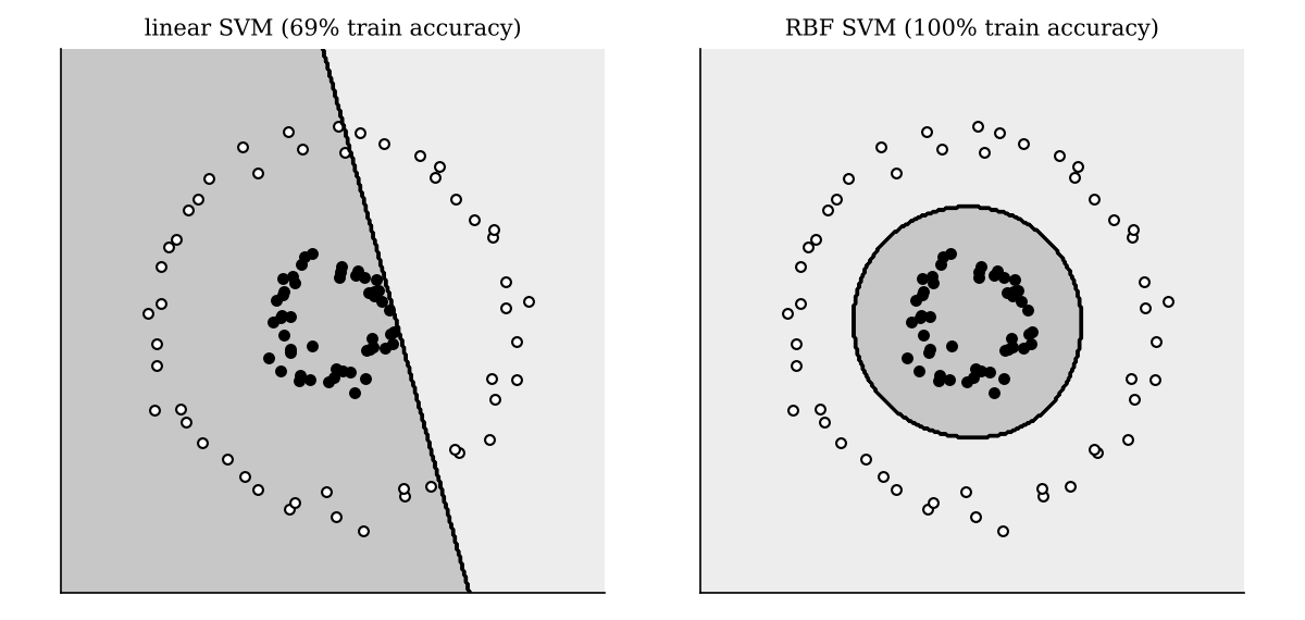
Somewhat surprisingly, despite the enormous flexibility of the RBF kernel, the learned boundary is a simple, almost circular curve, not a wildly overfit one. It has the right level of complexity for this data.
Why? The SVM does implicit regularization. Maximizing the margin means minimizing \(\|w\|^2\), the same penalty on model complexity as ridge regression in Chapter 1.3. So even though the model class is very rich, the SVM favors simple solutions within it. This is one of the reasons support vector machines were the star of machine learning before the deep learning era.