This chapter finishes deriving PCA, then visualizes what it does.
Where we left off. We want to embed data \(x_1, \dots, x_n \in \mathbb{R}^d\) into \(\mathbb{R}^k\) with a matrix \(U \in \mathbb{R}^{k \times d}\) with orthonormal rows, encoding with \(U\) and decoding with \(U^\top\), so as to minimize the reconstruction error. For \(k = 1\), this became \[ \max_{u_1} \|Xu_1\|^2 \quad \text{where } u_1 \in \mathbb{R}^d,\ \|u_1\| = 1. \] With the SVD \(X = W\Sigma V^\top\), we found that \(X\) acts very simply on the columns of \(V\): \(Xv_j = \sigma_j w_j\).
Express \(u_1 \in \mathbb{R}^d\) in the basis \(\{v_1, \dots, v_d\}\). The \(v_j\) are orthonormal, so they form a basis of \(\mathbb{R}^d\), and we can write \[ u_1 = \sum_{j=1}^d \alpha_j v_j \quad \text{for some } \alpha_1, \dots, \alpha_d \in \mathbb{R}, \qquad \sum_{j=1}^d \alpha_j^2 = 1. \] The constraint on the coefficients comes from \(\|u_1\| = 1\).
Our goal is to find \(\alpha_1, \dots, \alpha_d\) that maximize \(\|Xu_1\|^2\). Plug in, and use linearity to move \(X\) next to each \(v_j\): \[ \|Xu_1\|^2 = \Big\| X\Big(\sum_{j=1}^d \alpha_j v_j\Big) \Big\|^2 = \Big\| \sum_{j=1}^d \alpha_j (Xv_j) \Big\|^2. \] Now use \(Xv_j = \sigma_j w_j\). Here \(\alpha_j\) and \(\sigma_j\) are scalars and \(w_j\) is a vector, so group the scalars: \[ = \Big\| \sum_{j=1}^d \alpha_j (\sigma_j w_j) \Big\|^2 = \Big\| \sum_{j=1}^d (\alpha_j \sigma_j)\, w_j \Big\|^2. \] Apply the definition of the squared norm, \(\|v\|^2 = v^\top v\): \[ = \Big( \sum_{j=1}^d (\alpha_j \sigma_j)\, w_j \Big)^\top \Big( \sum_{j=1}^d (\alpha_j \sigma_j)\, w_j \Big) = \Big( \sum_{j=1}^d (\alpha_j \sigma_j)\, w_j^\top \Big) \Big( \sum_{j=1}^d (\alpha_j \sigma_j)\, w_j \Big). \] Expanding this product gives \(d^2\) terms, one for each pair of indices:
So all the cross terms vanish, and \[ \|Xu_1\|^2 = \sum_{j=1}^d (\alpha_j \sigma_j)^2. \]
So we have \[ \max_\alpha \sum_{j=1}^d \alpha_j^2 \sigma_j^2 \quad \text{with} \quad \sum_{j=1}^d \alpha_j^2 = 1. \] The singular values are given to us, already sorted with \(\sigma_1\) the largest. We have a total “budget” of 1 to split among the \(\alpha_j^2\), and each unit of budget on \(\alpha_j^2\) is worth \(\sigma_j^2\). The best strategy is to put all of it on the largest one: \[ \Rightarrow\quad \alpha_1^* = 1, \qquad \alpha_2^* = \alpha_3^* = \dots = \alpha_d^* = 0. \] In other words, \(u_1 = v_1\), the first right singular vector of \(X\). Translating back to the original problem, \[ \Rightarrow\quad \operatorname*{argmin}_{UU^\top = 1} \sum_{i=1}^n \|x_i - U^\top U x_i\|^2 = \big[\; \text{---}\; v_1^\top \;\text{---} \;\big]. \]
The same logic extends to larger \(k\). The best \(k\)-dimensional embedding uses the first \(k\) rows of \(V^\top\): the \(k\) directions that \(X\) stretches the most.
Setup (principal component analysis)
\(Ux \in \mathbb{R}^k\) are called the “principal components” of \(x \in \mathbb{R}^d\): the first \(k\) principal components. In practice, \(Ux\) is all you need to use PCA. The derivation is how we know these components are the right ones.
Why center the data? Centering is a standard preprocessing step for PCA, much like bias lifting for regression. Without centering, PCA still minimizes reconstruction error. After centering, the objective gains a second interpretation: minimizing reconstruction error is the same as maximizing the variance of the projected data. The principal components are the directions that preserve as much of the data’s variance as possible. You will show this in Homework 3.
Notation and interpretation:
To see the geometry of encoding and decoding, we embed a 2D dataset into 1D. You would never use PCA for this in practice, but it is the only case we can draw. We simulate 50 centered points in \(\mathbb{R}^2\):
np.random.seed(4721)
X = np.random.multivariate_normal([0, 0], [[0.4, 0.28], [0.28, 0.25]], size=50)
X = X - X.mean(axis=0)              # center the data
To embed in 1D, we need \(U \in \mathbb{R}^{1 \times 2}\) with orthonormal rows, which is the same as a unit vector \(u \in \mathbb{R}^2\). Pick any vector and normalize it:
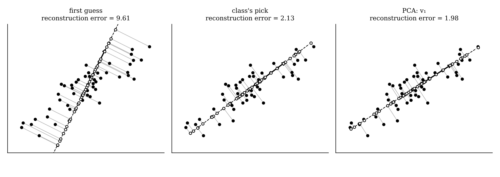
u = np.array([1, 2]) / np.linalg.norm([1, 2]) # a first guessEach reconstruction \(\hat x_i\) is the orthogonal projection of \(x_i\) onto the line spanned by \(u\). That is why \(U^\top U\) is often called a projection matrix. The reconstruction error \(\|x_i - \hat x_i\|^2\) is the squared length of the segment connecting a point to its projection.
In each panel, filled dots are the original points, hollow dots are their reconstructions, gray segments show each point’s error, and the dashed line is the subspace spanned by \(u\). Read the linear algebra off the picture:
Question: can you pick a different direction that reduces the reconstruction error?
The first guess (left) has a total reconstruction error of about 9.61. A direction picked by eye in class, along the data’s long axis with slope \(0.75\), i.e. \(u = (0.8, 0.6)\), does much better: about 2.13. And PCA’s answer, \(v_1\) from the SVD (right), is the best possible, at about 1.98. Notice that PCA’s direction is the one along which the data are most spread out. That is the “maximum variance” interpretation.
Now a real dataset: images of handwritten digits. Each image is \(8 \times 8\) pixels, represented as a vector in \(\mathbb{R}^{64}\) where each entry stores a pixel value.

We construct \(U \in \mathbb{R}^{2 \times 64}\) by:
from sklearn.datasets import load_digits
X = load_digits().data
X = X - X.mean(axis=0, keepdims=True)

W, S, Vt = np.linalg.svd(X)
U = Vt[:2, :]                 # shape (2, 64)
embeddings = X @ U.T          # shape (n, 2): z_i = U x_i for every image
The first entry of \(Ux\) stores \(v_1 \cdot x\), and the second stores \(v_2 \cdot x\): how much of image \(x\) lies in each of two directions in pixel space.
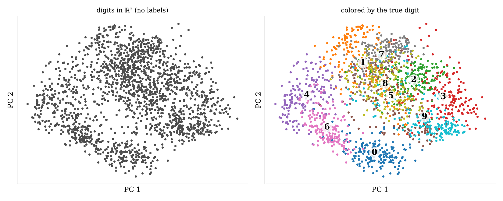
Is this embedding meaningful? On the left, PCA never saw the labels. On the right, we color each point by its true digit. Even with only 2 of the original 64 dimensions, images of the same digit tend to land near each other. 0s, 4s, 6s and 3s each occupy their own region, while some digits, like 1, 7 and 8, overlap. PCA found this structure without any supervision.