Last time: we found a good dimensionality-reducing transformation, one that minimizes the reconstruction loss, by restricting to linear maps with orthonormal rows and using the SVD.
Today: a different unsupervised task. Instead of finding a new representation of the data, we stay in the original space and look for structure: we partition the data into meaningful “structures.” Different notions of structure lead to different algorithms. Here we look at the most common one, clustering.
Task (clustering). Given \(x_1, \dots, x_n \in \mathbb{R}^d\) and a target number of clusters \(k\), find cluster assignments \[ c_1, \dots, c_n \in [k], \] where \([k] := \{1, \dots, k\}\). Each \(c_i\) says which of the \(k\) clusters point \(x_i\) belongs to.
Note that \(k\) now means the number of clusters, not the embedding dimension from PCA. We will use \([k]\) often.
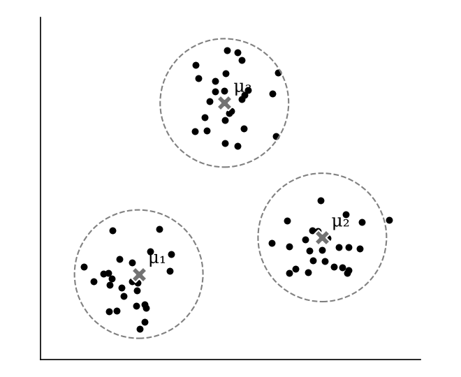
Look at the data above. If someone told you there are three clusters, most people would group the points the same way. The idea of k-means is to describe each group by a single point at its center.
Write \(S_j := \{i : c_i = j\}\) for the indices of the points assigned to cluster \(j\). For example, \(S_1 = \{1, 2, 10, 11, 20, 200\}\) lists the points in cluster 1.
Idea. Find a set of centers, or representatives, \(\mu_1, \dots, \mu_k \in \mathbb{R}^d\) such that each \(x_i\) is close to one center.
If \(\mu_1, \dots, \mu_k \in \mathbb{R}^d\) are given, the assignments are easy: assign each point to its closest center, \[ c_i \leftarrow \operatorname*{argmin}_{j \in [k]} \|x_i - \mu_j\|^2. \]
So the real challenge is finding good centers. A natural cost for a set of centers adds up, over all points, the squared distance from each point to its closest center. If a point were assigned to a faraway center, that term would be large. So we find \(\mu_1, \dots, \mu_k \in \mathbb{R}^d\) that solve \[ \min_{\mu_1, \dots, \mu_k \in \mathbb{R}^d} \sum_{i=1}^n \min_{j \in [k]} \|x_i - \mu_j\|^2. \]
Remark. Solving this optimization problem is NP-hard. We’ll approximate it using Lloyd’s algorithm.
Why is it so hard? There are two nested problems. The outer minimization is over the centers, which are continuous variables; that part alone would be manageable with descent-type methods. But the inner minimization is over discrete assignments. Optimizing over discrete choices is a combinatorial problem, and without special structure, the best general approach is close to exhaustive search.
We just saw that given the centers, finding the assignments is easy. The reverse is easy too: given the assignments, what is a good representative for each cluster? Its mean. Lloyd’s algorithm alternates between these two easy steps, which is where the name k-means comes from.
Algorithm (Lloyd’s algorithm). Given data \(x_1, \dots, x_n \in \mathbb{R}^d\) and an intended number of clusters \(k\):
Moving the centers can change the assignments, and changing the assignments moves the centers, so we alternate until nothing changes, then output the assignments. If a point is exactly equidistant from two centers, break the tie arbitrarily.
k-means compares each point with the centers, never with other points. So two points that are very close to each other can still be assigned to different clusters, if they sit on either side of the boundary halfway between two centers. k-means only guarantees that each point is assigned to its closest center.
Run k-means with \(k = 2\) clusters on four points on the real line: \(x_1 = 1\), \(x_2 = 2\), \(x_3 = 8\), \(x_4 = 9\). Here \(n = 4\) and \(d = 1\).
Setup (k-means)
Remarks.
This is different from most algorithms we have seen. Even without a closed form, gradient descent on a convex loss reaches a global optimum. k-means has no such guarantee, so if you run it once and get a result, don’t simply trust it.
We generate a 2D dataset with three groups of very different sizes (300, 30 and 30 points), centered at \((0, 0)\), \((5, 0)\) and \((10, 0)\), and run Lloyd’s algorithm from two initializations. Gray × marks show the initial centers; black ✖ marks show where they converge.
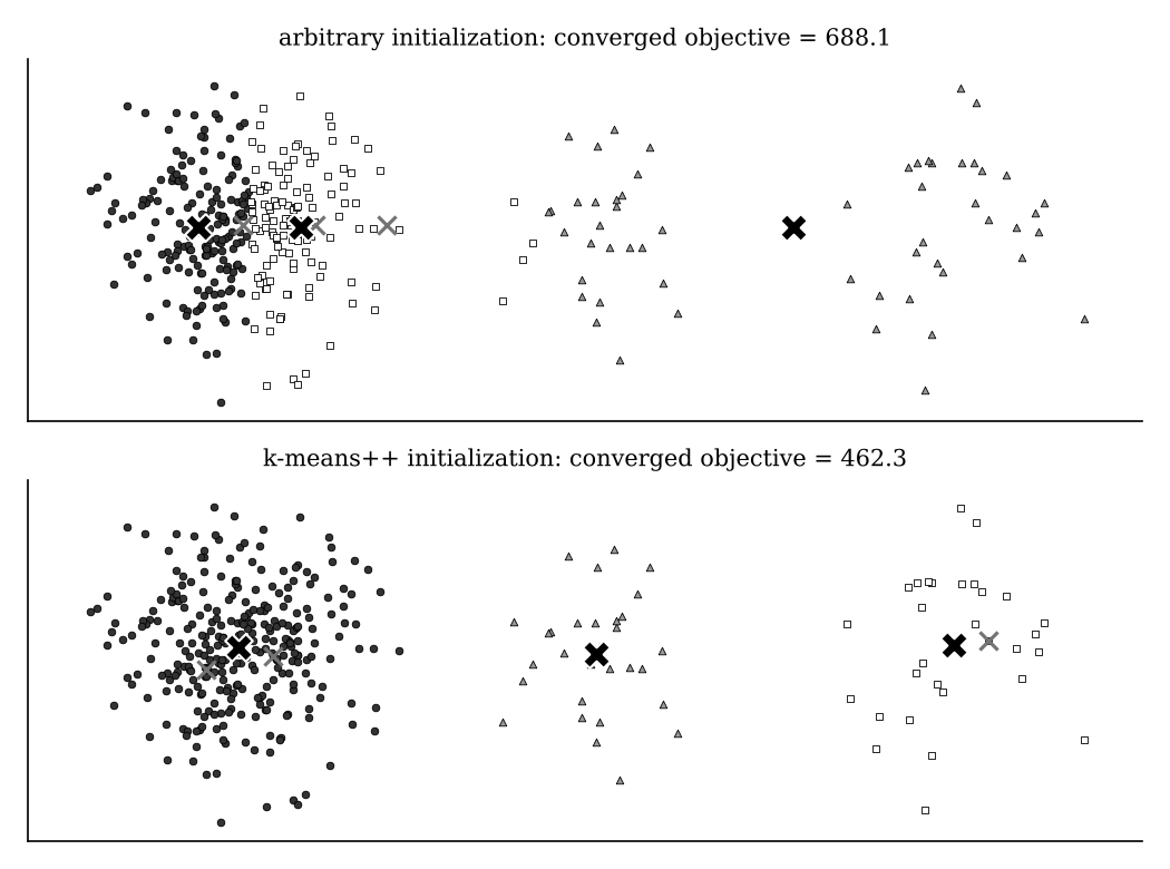
A bad local optimum can happen. With an arbitrary initialization at \((0, 0)\), \((1, 0)\) and \((2, 0)\), all three centers start inside the big group. Lloyd’s algorithm makes some progress: the third center moves right, toward the two small groups. But it gets stuck after 5 rounds with the big group split in two and the two small groups merged. The objective is 688.1. It can make small local adjustments, but it cannot escape this choice of centers.
A better initialization: k-means++. The basic idea of k-means++ is to spread the initial centers across the dataset. Here one center starts far to the right. It takes more rounds (12), but the two right-hand centers gradually separate, and Lloyd’s algorithm converges to the clustering a human would choose, with a much lower objective of 462.3. You could also start from random assignments instead of random centers; what ultimately matters is where the centers end up.
k-means requires us to choose \(k\) in advance. In supervised learning we would use cross-validation, but with no labels, choosing hyperparameters for unsupervised methods is much less clear-cut. (Homework 3 gives one way to choose the embedding dimension for PCA.)
Will the objective ever go up as \(k\) increases? No. With one more center, you can always split an existing cluster and move the two centers closer to their points. In the extreme, with \(k = n\) clusters, every point is its own center and the objective is \(0\): a perfect score, and a useless clustering. So the objective always decreases as \(k\) grows, and we cannot just pick the \(k\) with the smallest objective.
A common heuristic is the elbow method:
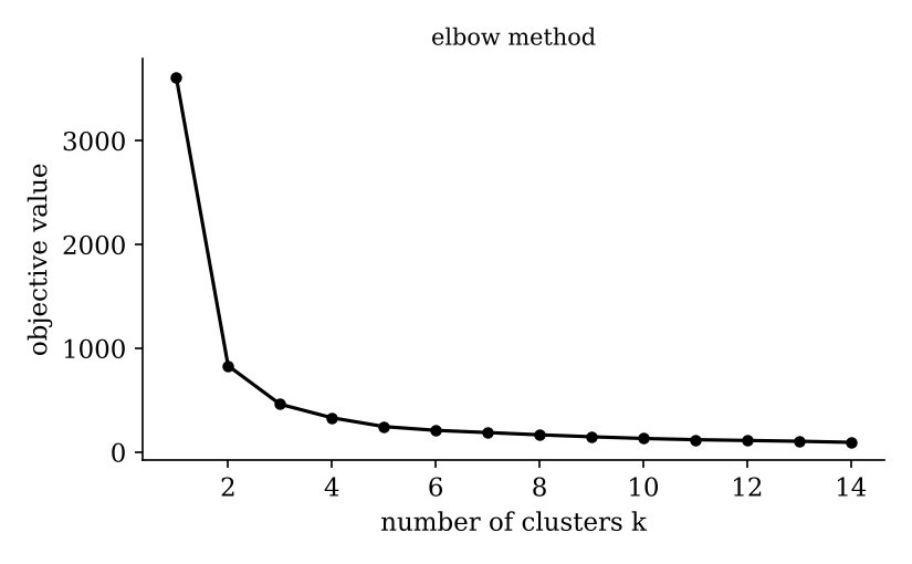
For the dataset above, the objective drops sharply from \(k = 1\) to \(k = 2\), then by smaller amounts to \(k = 3\) and \(k = 4\), and after that the decrease is so gentle that it probably reflects noise rather than real structure. Reading an elbow plot is subjective: someone arguing for 2, 3 or 4 clusters here would have a reasonable case, while 100 clusters would not.
In practice, domain knowledge is also important: what number of clusters is useful for the application? For example, if you know a blood sample contains about 10 cell types, cluster single-cell data from it into about 10 clusters. Like many choices in data science, this is a design decision you have to make and take responsibility for.
Next time: k-means gives a hard assignment, with each point in exactly one cluster. Next, a probabilistic clustering model that lets us reason about uncertainty in the cluster assignments.