Last time: k-means clustering. Given the centers, assigning points is easy (pick the closest center). Given the assignments, updating the centers is easy (take the mean). Lloyd’s algorithm alternates between the two.
But k-means gives each point a single label, even when we shouldn’t be confident about it. Take two points that sit right in the middle between two centers: k-means may put them in different clusters, and its output does not tell us that either assignment is a close call.
Today: a probabilistic version of clustering. Instead of a single label in \([k]\), each point gets a probability distribution over the \(k\) clusters, so the model’s uncertainty about the assignment is part of the output. To do this, we first write down a probabilistic model of how clustered data is generated, and then derive an algorithm that reverses that process.
When you draw a clustered dataset by hand, you naturally do it in two stages: first you decide which cluster you’re drawing in, then you put a point somewhere near that cluster’s center. The Gaussian mixture model (GMM) turns this into a probability model.
Model (GMM)
Each piece of the model has a role:
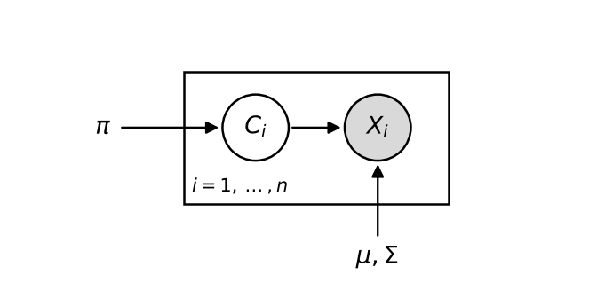
As a diagram, with the observed variable shaded:
The box means the same structure repeats for every data point \(i = 1, \dots, n\). The parameters \(\pi\), \(\mu\) and \(\Sigma\) sit outside the box because they are shared by all points.
Start with the simplest interesting case: points on the real line, two clusters. Consider the following GMM:
(In one dimension, \(\Sigma_j\) is just the variance.)
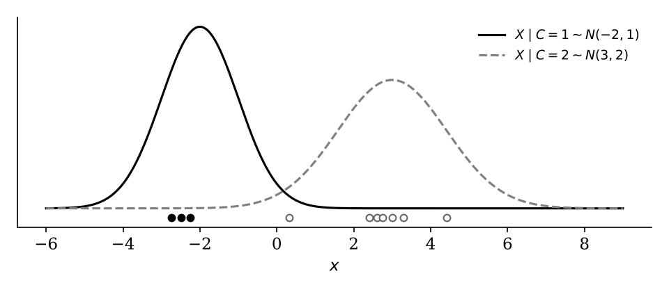
To sample 10 points from this model, we would draw about 4 of them from the first Gaussian (filled dots) and about 6 from the second, which is wider (open dots). Our task is to reverse this process: someone shows us only the 10 dots, with no fill, and asks which distribution each one came from.
Check your understanding. How many numbers do you need to specify \(\text{Discrete}(\pi_1, \dots, \pi_k)\)?
\(k - 1\). The probabilities must sum to 1, so once \(\pi_1, \dots, \pi_{k-1}\) are chosen, \(\pi_k\) is determined. In the example, choosing \(\pi_1 = 0.4\) forces \(\pi_2 = 0.6\).
Task (probabilistic clustering). Find \[ w_i^{(j)} \in (0, 1), \qquad i = 1, \dots, n, \quad j = 1, \dots, k, \] the probability of data point \(x_i\) being in cluster \(j\). For each \(i\), the \(k\) numbers \(w_i^{(1)}, \dots, w_i^{(k)}\) sum to 1. We index data points by \(i\) and clusters by \(j\) throughout.
In the figure above, a point near \(-2\) might get weights \(w = (0.9, 0.1)\), and a point near \(2\) might get \(w = (0.2, 0.8)\).
We borrow the idea behind k-means: split the problem into two halves that are each easy.
Idea, part 1: if the model parameters \(\theta\) are given. Then computing the weights is easy: \[ w_i^{(j)} \leftarrow \frac{\pi_j \, p_\theta(x_i \mid j)}{\sum_{j' \in [k]} \pi_{j'} \, p_\theta(x_i \mid j')}, \] where \(p_\theta(x_i \mid j)\) is the density of \(N(\mu_j, \Sigma_j)\) evaluated at \(x_i\).
This is Bayes’ rule, and both factors in the numerator matter.
The numerator is the joint density of \(x_i\) and cluster \(j\). Dividing by the sum over all clusters makes the weights for point \(i\) add up to 1.
Idea, part 2: if the soft assignments \(w_i^{(j)}\) are given. Then estimating the parameters is easy too. Think of \(w_i^{(j)}\) as the amount of point \(i\) that belongs to cluster \(j\):
Idea. Alternate between
Algorithm (Expectation Maximization). Given data \(x_1, \dots, x_n \in \mathbb{R}^d\) and an intended number of groups \(k\):
The names come from statistics: the E-step computes the expected cluster memberships under the current model, and the M-step maximizes the likelihood of the model given those memberships. The denominators in \(\mu_j\) and \(\Sigma_j\) normalize by the total weight assigned to cluster \(j\), just as k-means divides by \(|S_j|\).
The stopping rule is different from Lloyd’s algorithm. There, the assignments were discrete, so they eventually stopped changing. Here, the weights are continuous and will almost never stop moving exactly, so we stop once the changes fall below a small tolerance.
Run EM on four points on the real line: \(x_1 = 1\), \(x_2 = 2\), \(x_3 = 5\), \(x_4 = 8\).
Initialize the parameters: \[ \pi_1 \leftarrow \tfrac12, \quad \mu_1 \leftarrow 3, \quad \Sigma_1 \leftarrow 1; \qquad \pi_2 \leftarrow \tfrac12, \quad \mu_2 \leftarrow 4, \quad \Sigma_2 \leftarrow 1. \] That is, we start by assuming the two clusters are equally likely and equally spread out, with centers at 3 and 4.
Expectation step. Fix \(\theta\): \[ C_i \sim \text{Discrete}(\tfrac12, \tfrac12), \qquad X_i \mid C_i = 1 \sim N(3, 1), \qquad X_i \mid C_i = 2 \sim N(4, 1). \] There are \(4 \times 2 = 8\) weights to compute. Let’s compute \(w_4^{(1)}\) and \(w_4^{(2)}\), for the last point, \(x_4 = 8\). Plugging into the Gaussian density \(p(x) = \frac{1}{\sqrt{2\pi\Sigma}} e^{-(x - \mu)^2 / (2\Sigma)}\): \[ p_\theta(X_4 = 8 \mid C_4 = 1) = \tfrac{1}{\sqrt{2\pi}} e^{-25/2} \approx 1.5 \times 10^{-6}, \qquad p_\theta(X_4 = 8 \mid C_4 = 2) = \tfrac{1}{\sqrt{2\pi}} e^{-16/2} \approx 1.3 \times 10^{-4}. \] So \[ w_4^{(1)} \approx \frac{\tfrac12 (1.5 \times 10^{-6})}{\tfrac12 (1.5 \times 10^{-6}) + \tfrac12 (1.3 \times 10^{-4})} \approx 0.011, \qquad w_4^{(2)} \approx 0.989. \] The point at 8 is far from both centers, but it is much farther from 3 than from 4, so nearly all its weight goes to cluster 2. The same computation for the other points gives:
| \(i\) | \(x_i\) | \(w_i^{(1)}\) | \(w_i^{(2)}\) |
|---|---|---|---|
| 1 | 1 | 0.924 | 0.076 |
| 2 | 2 | 0.818 | 0.182 |
| 3 | 5 | 0.182 | 0.818 |
| 4 | 8 | 0.011 | 0.989 |
Maximization step. Fix the \(w_i^{(j)}\) and update \(\mu_j\), \(\pi_j\), \(\Sigma_j\). For the means: \[ \mu_1 \leftarrow \frac{0.924(1) + 0.818(2) + 0.182(5) + 0.011(8)}{0.924 + 0.818 + 0.182 + 0.011} \approx 1.84, \qquad \mu_2 \leftarrow 6.02. \] The two centers move apart, toward the two groups of points. The other parameters update to \(\pi \approx (0.48, 0.52)\) and \(\Sigma \approx (1.50, 4.64)\). The second cluster becomes much wider, because it has to account for both 5 and 8.
Repeating the two steps, EM converges after 14 rounds to \(\pi \approx (0.50, 0.50)\), \(\mu \approx (1.50, 6.48)\) and \(\Sigma \approx (0.25, 2.33)\). In the final model, points 1 and 2 belong to cluster 1 with probability above 0.99, and points 3 and 4 belong to cluster 2.
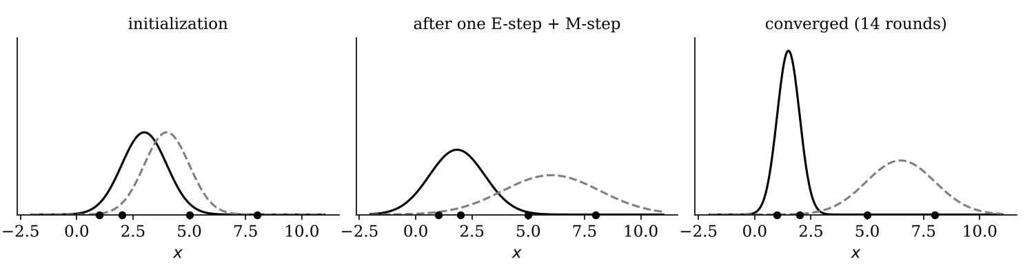
Each curve shows \(\pi_j \, p(x \mid j)\), the cluster’s density scaled by its prior.
Setup (Gaussian mixture modeling)
Remark. Similar to Lloyd’s algorithm, the output of the EM algorithm also depends on initialization and can converge to a poor solution. In practice, people run EM from several initializations, or initialize it from the output of k-means.
Lloyd’s algorithm is a “hard” version of EM. If every \(w_i^{(j)}\) were forced to be 0 or 1 (all weight on the most likely cluster), and all clusters had the same prior and the same spherical covariance, the E-step would assign each point to its nearest center, and the M-step update for \(\mu_j\) would become the mean of the points in cluster \(j\). Those are exactly Lloyd’s two steps. The GMM adds two things: soft assignments, and clusters with their own sizes (\(\pi_j\)) and shapes (\(\Sigma_j\)).
We generate two overlapping groups of 150 points in 2D and cluster
them with k-means and with a two-component GMM (scikit-learn’s
GaussianMixture, which runs EM).
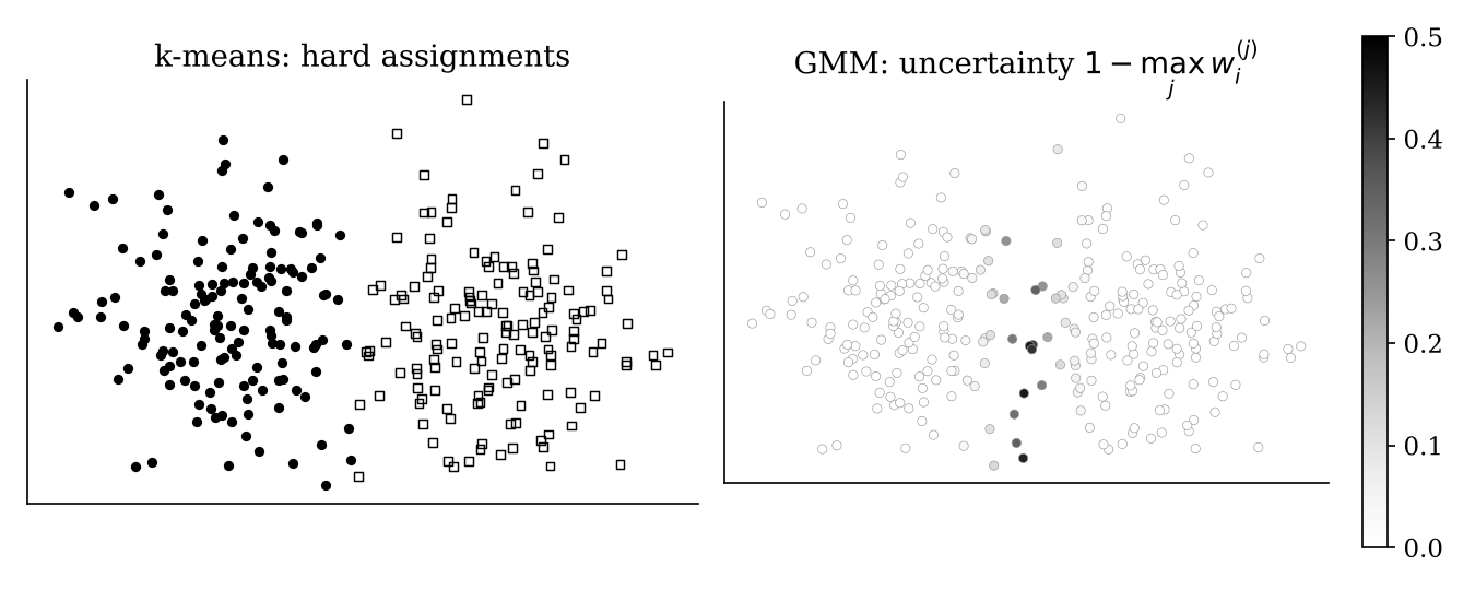
k-means (left) draws a sharp boundary: every point gets one label, including the ones in the overlap. The GMM recovers almost the same two clusters, but it also tells us where it is unsure (right). Most points have uncertainty near 0, while about a dozen points in the overlap region are close to 50/50. Those are exactly the points whose k-means labels we should not trust.
In scikit-learn, GaussianMixture(n_components=k).fit(X)
runs EM, and .predict_proba(X) returns the \(n \times k\) matrix of weights \(w_i^{(j)}\). Try changing
covariance_type ("full", "diag",
"spherical") to control the shapes the clusters can
take.