This is the last module: deep learning. In the earlier modules, we usually spent a little time defining a model and a lot of time deriving its learning algorithm. This module flips that. Today we learn one general way to train neural networks, and after that we spend most of our time on how to design a good model, or as people say in deep learning, a good architecture.
Recall: the perceptron. In 2.5 we studied the perceptron model:
Drawing each number as a circle, the perceptron combines the \(d\) input coordinates into a single number using the weights and the bias, and then takes the sign. But this model class is quite limited: it cannot even learn the XOR function. At the end of 2.5, we previewed the fix: combine several perceptrons.
Instead of combining the inputs into a single number once, we do it \(m\) times, using \(m\) perceptron-like units, and then combine their outputs at the end.
Hyperparameters:
Model:
Parameters:
Each hidden unit needs its own weight vector in \(\mathbb{R}^d\) and its own bias, as a perceptron does. Stacking the \(m\) weight vectors as rows gives the matrix \(W\), and stacking the biases gives the vector \(b\). Check the shapes: \(W\) is \(m \times d\) and \(x\) is in \(\mathbb{R}^d\), so \(Wx + b \in \mathbb{R}^m\), one number per hidden unit. The output layer is a small regression on top of the hidden layer: \(a\) and \(c\) combine the \(m\) hidden outputs into a single prediction \(\hat y \in \mathbb{R}\). For now we focus on regression, so the output is a real number.
This small change makes a big difference. An MLP with a single hidden layer can approximate any “reasonable” function, provided it has enough hidden units. “Reasonable” is in quotes, but it covers essentially every function we have worked with, XOR included.
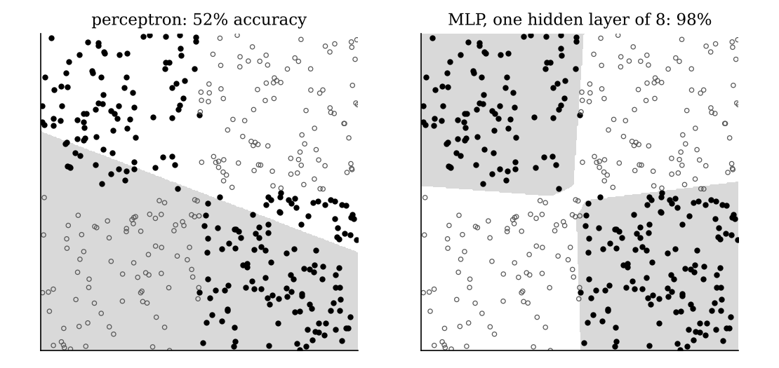
The figure above shows this on XOR-style data, where the label depends on whether the two coordinates have the same sign. A perceptron can only draw one line, so it does little better than guessing (52%). An MLP with one hidden layer of 8 ReLU units fits the data almost perfectly (98%).
Idea. What if we go deeper?
If one hidden layer can already approximate any reasonable function, why add more? The catch is how many units it takes. To represent some functions with a single hidden layer, the number of hidden units has to grow exponentially, which is impractical. Adding more hidden layers lets a network represent complex functions with far fewer units in total. This is the motivating idea of deep learning, as opposed to shallow learning.
To add a layer, we do the same thing again: map the output of one hidden layer to the next using a weight matrix, a bias and a nonlinearity. If \(h_1\) has \(m_1\) entries and \(h_2\) has \(m_2\) entries, the matrix that maps \(h_1\) to \(h_2\) must be \(W_2 \in \mathbb{R}^{m_2 \times m_1}\). For example, to map two numbers to three numbers, we need a \(3 \times 2\) matrix. The first dimension is always the output dimension.
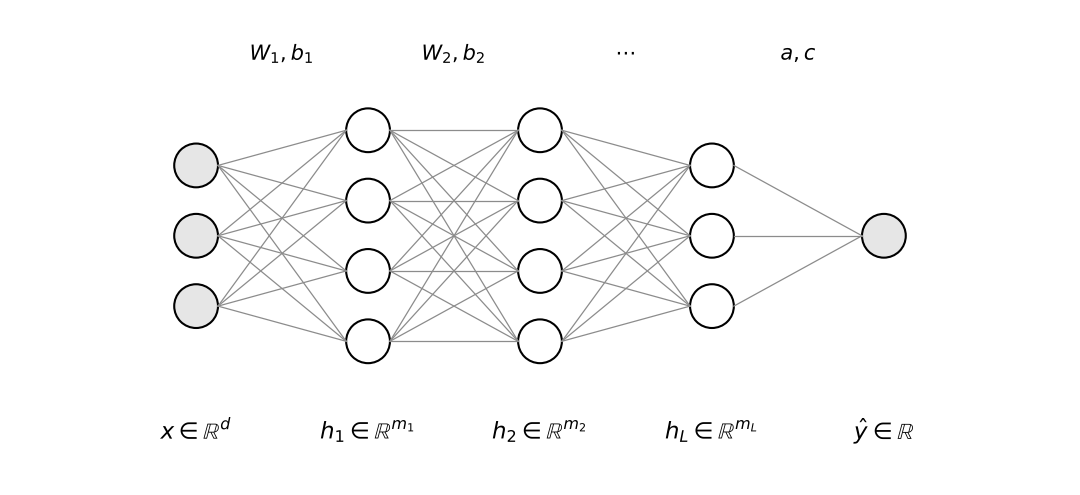
Model (multilayer perceptron)
Hyperparameters:
Model:
Parameters:
Each layer reads the output of the previous layer, multiplies it by a weight matrix, adds a bias, and applies the nonlinearity. Why do we need \(\sigma\)? Without it, every layer would be a linear map (plus a shift), and a composition of linear maps is still linear. However deep the network, it could only represent linear functions.
If the formulas feel hard to reason about, focus on the picture. It’s worth being able to write the model down precisely, but the diagram carries the same information.
The parameters are learned from data. The hyperparameters, the number of layers and units and the choice of \(\sigma\), are decided in advance. For the simpler models in this course, we chose hyperparameters by cross-validation. For deep networks there are so many choices that trying them all isn’t practical. Instead, practitioners follow guidelines that depend on the application, and that is what most of this module is about.
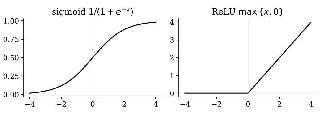
There are many other activations, each with its pros and cons. For example, ReLU has no derivative at 0, so smooth versions such as GELU are also popular. For this course, sigmoid and ReLU are enough.
Hyperparameter: \(\sigma_{\text{ReLU}}(x) = \max(x, 0)\) as the activation. The picture fixes the others: one hidden layer (\(L = 1\)) with two hidden units (\(m_1 = 2\)), and inputs \(x \in \mathbb{R}^2\).
Whenever you meet new notation, first ask: is it a number, a vector or a matrix, and what are its dimensions? Here \(W_1 \in \mathbb{R}^{2 \times 2}\) maps the 2-dimensional input to 2 hidden units, and \(b_1 \in \mathbb{R}^2\) has the same dimension as the hidden layer. The output weights \(a \in \mathbb{R}^2\) play the role of a perceptron’s weights on top of the hidden layer, and \(c \in \mathbb{R}\) is a single number.
Model:
As in the first half of the GMM lecture, these parameter values are given to us so we can see how the model works. Later, they will be learned from data.
Forward pass. What does the model output for \(x = \begin{bmatrix} 1 \\ 0 \end{bmatrix}\)?
These are ideas we already know, applied to a much richer class of models. The rest of the module answers them:
| lecture | architecture | used for |
|---|---|---|
| 4.1 | MLP (1986) | general architecture |
| 4.2 | CNN (1989) | images |
| 4.3 | Autoencoder (2006) | unsupervised learning |
| 4.4 | Transformer (2017) | sequences |
Today we answer the first question, for the general MLP architecture. The same training procedure works for every architecture that follows.
We take the average rather than the sum, which is helpful for technical reasons but measures the same thing: the average quality of our predictions. A neural network is far too complex to hope for a closed-form solution. And because the objective is non-convex, we can only hope to approximate a solution.
Approximate a solution using gradient descent:
The problem is computation. Neural networks shine when \(n\) is large, and every gradient step here requires a pass over the entire dataset. The fix: approximate the gradient using a single data point.
The gradient at a single data point is a noisy estimate of the full gradient, which is why the method is called stochastic. In practice, we loop over the dataset this way, possibly several times.
Initializing is easy, and so is subtracting a scaled vector. The hard part is the gradient itself. A neural network applies a long chain of operations to its input, so we compute the gradient using the chain rule. Applied to neural networks, this is called backpropagation (“backprop”).
Backprop is a little like eating spinach: not the most exciting thing you’ll do, but good for you. You should work through at least one example by hand to understand how a network is trained.
We use the same tiny network as before.
The network is defined by \(h_1 = \sigma_{\text{ReLU}}(W_1 x + b_1)\) and \(\hat y = a \cdot h_1 + c\). From the forward pass, \(h_1 = (1, 1)\) and \(\hat y = 2\). The true label is 1, so we want to move the four parameters so that the prediction moves toward 1.
We compute the gradients backwards: first for the output layer (\(a\), \(c\)), then for the hidden layer (\(W_1\), \(b_1\)). Working backwards lets us reuse what we have already computed. It helps to keep track of the derivatives of the loss with respect to each layer’s output (\(\hat y\) and \(h_1\)), because those get reused.
Start with the loss itself. \[ \frac{\partial l}{\partial \hat y} = 2(\hat y - y) = 2(2 - 1) = 2. \]
Output weights \(a\). The loss doesn’t depend on \(a\) directly, only through \(\hat y\), so we apply the chain rule. Since \(\hat y\) depends linearly on \(a\), \(\partial \hat y / \partial a = h_1\): \[ \frac{\partial l}{\partial a} = \frac{\partial l}{\partial \hat y} \frac{\partial \hat y}{\partial a} = 2 h_1 = \begin{bmatrix} 2 \\ 2 \end{bmatrix}. \]
Output bias \(c\). This one is a single number, like \(c\) itself. The gradient always has the same shape as the parameter: \[ \frac{\partial l}{\partial c} = \frac{\partial l}{\partial \hat y} \frac{\partial \hat y}{\partial c} = 2 \cdot 1 = 2. \]
The hidden layer output \(h_1\). This one we keep, because the last two gradients need it: \[ \frac{\partial l}{\partial h_1} = \frac{\partial l}{\partial \hat y} \frac{\partial \hat y}{\partial h_1} = 2a = \begin{bmatrix} 2 \\ 2 \end{bmatrix}. \]
Hidden weights \(W_1\). This is a \(2 \times 2\) matrix. To see how \(h_1\) changes with \(W_1\), we need the derivative of ReLU: \[ \frac{\partial \sigma_{\text{ReLU}}(z)}{\partial z} = \begin{cases} 0 & z < 0, \\ 1 & z > 0. \end{cases} \] (It is undefined at exactly \(z = 0\).) Here both entries of \(W_1 x + b_1 = (1, 1)\) are positive, so ReLU passes them through unchanged, and \(h_1\) is just \(W_1 x + b_1\) locally. That depends linearly on \(W_1\), which gives a factor of \(x\). To get a \(2 \times 2\) result from a vector in \(\mathbb{R}^2\), it must be \(x^\top\): \[ \frac{\partial l}{\partial W_1} = \frac{\partial l}{\partial h_1} \frac{\partial h_1}{\partial W_1} = \begin{bmatrix} 2 \\ 2 \end{bmatrix} x^\top = \begin{bmatrix} 2 \\ 2 \end{bmatrix} \begin{bmatrix} 1 & 0 \end{bmatrix} = \begin{bmatrix} 2 & 0 \\ 2 & 0 \end{bmatrix}. \] If you’re unsure about a transpose, check the shapes: you know what shape the answer must have.
Hidden bias \(b_1\). Same idea, and \(\partial h_1 / \partial b_1\) is 1 in each coordinate here: \[ \frac{\partial l}{\partial b_1} = \frac{\partial l}{\partial h_1} \frac{\partial h_1}{\partial b_1} = \begin{bmatrix} 2 \\ 2 \end{bmatrix}. \]
With learning rate \(\eta = 0.1\), the updates are \(a \leftarrow (0.8, 0.8)\), \(c \leftarrow -0.2\), \(W_1 \leftarrow \begin{bmatrix} 0.8 & 1 \\ 0.8 & 1 \end{bmatrix}\) and \(b_1 \leftarrow (-0.2, -0.2)\). A new forward pass gives \(W_1 x + b_1 = (0.6, 0.6)\), \(h_1 = (0.6, 0.6)\), and \(\hat y = 0.8(0.6) + 0.8(0.6) - 0.2 = 0.76\). The prediction moved from 2 to 0.76, and the loss dropped from 1 to about 0.06. (The step overshot the target a little; a smaller \(\eta\) would move more cautiously.)
This is a general technique. For any other architecture, backprop works the same way: compute the gradients layer by layer, from the output back to the input, reusing what you’ve already computed. We won’t do it by hand again, but you should be able to.
Redo this example without looking at the solution. Then make your own practice problem with different values. For instance, choose an input for which one of the hidden units has a negative pre-activation, and see what ReLU does to its gradients.