Last time: the multilayer perceptron (also called an artificial neural network). The name comes from biology: the model was loosely inspired by how neurons in the brain pass information along.
In an MLP, every layer is a dense layer: a full matrix connects every neuron in one layer to every neuron in the next. Going from \(d\) neurons to \(m_1\) neurons takes an \(m_1 \times d\) matrix, one parameter per pair of neurons.
We left one question open: how do we pick the hyperparameters? Today we answer it for one important application: images.
Convolutional neural networks are neural networks that use convolution instead of general matrix multiplication in at least one of their layers. They have strong empirical performance when \(\mathcal{X}\) is a set of images.
Much of deep learning theory is still being worked out, so many design choices in this module come from experiments rather than proofs. Designing an architecture takes some creativity plus a lot of engineering.
Example: handwritten digit recognition. An image is a matrix of numbers, where each entry is the intensity of one pixel. Given an image of a handwritten digit, we want to predict its label in \(\{0, 1, 2, \dots, 9\}\). This was the first task on which deep learning, and CNNs in particular, reached human-level performance.
| input image | → | feature map #1 | → | feature map #2 | → | feature map #3 | → | feature map #4 | → | output |
|---|---|---|---|---|---|---|---|---|---|---|
| \(28 \times 28\) | convolution | \(6 \times 28 \times 28\) | pooling | \(6 \times 14 \times 14\) | convolution | \(16 \times 10 \times 10\) | pooling | \(16 \times 5 \times 5\) | MLP | \(10\) |
When you meet a new architecture, first ask what goes in and what comes out.
In between, the hidden outputs are called feature maps when we work with images. A convolution layer turns the single image into 6 feature maps. A pooling layer shrinks each one to \(14 \times 14\). A second convolution turns those into 16 smaller feature maps, and a second pooling shrinks them to \(5 \times 5\). Finally, the \(16 \times 5 \times 5 = 400\) numbers are flattened into one long vector, and an MLP maps it to the 10 outputs.
The end of the network is an MLP, which we already understand. The rest of this chapter explains the two new building blocks: convolution and pooling. To train the network, we use the same SGD + backprop as before.
Question: how do we build a layer when the inputs are 2D?
Idea: flatten the 2D input into a 1D vector, and then use an MLP. An MLP can approximate any reasonable function, so why not?
Issue: spatial information is lost. If we stack the rows of an image into one long vector, pixels that were directly above and below each other end up far apart, while the last pixel of one row lands right next to the first pixel of the next, even though they’re on opposite sides of the image. The MLP has no way of knowing which pixels were neighbors.
\(\implies\) We want an operation that is naturally defined on 2D inputs.
Better idea: use convolution instead of matrix multiplication to connect layers.
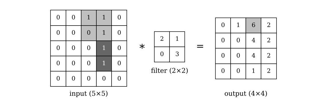
Think of the convolution filter as a small mask that we slide across the input. At each position, we multiply the filter element-wise with the patch of the input underneath it and add up the results, like a dot product. Each position gives one entry of the output.
Sliding across all \(4 \times 4\) positions gives the output shown. Check your understanding: compute the bottom row of the output yourself.
\(0, 0, 1, 2\). In the third position, only the filter’s top-right entry (\(1\)) sits on a nonzero pixel. In the fourth, only the top-left entry (\(2\)) does.
The filter values are parameters: they are learned from data. Notice how few there are. Mapping 25 numbers to 16 numbers with a matrix would take \(16 \times 25 = 400\) parameters. The convolution uses 4, and the same 4 numbers are reused at every position of the image.
Practical notes:
Before deep learning, people in image processing designed useful filters by hand. Some detect edges and others blur or sharpen. The figure shows three of them applied to a photo.
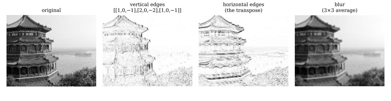
The idea of a CNN is to learn good filters from data, for whatever task the network is trained on.
Observation: there is a lot of redundant information in an image. Neighboring pixels are usually similar, so we can still tell what an image shows from a lower-resolution version.
Idea: reduce the resolution of the image to summarize it.
A pooling layer slides a window across the input, like convolution does. But instead of a learned filter, it summarizes each window with a fixed operation. Two common choices are:
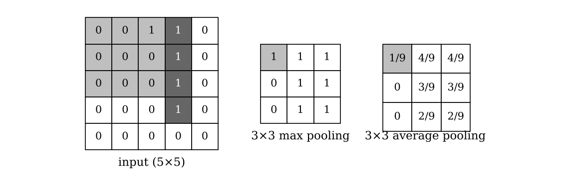
With a \(3 \times 3\) window moved one pixel at a time, a \(5 \times 5\) input becomes \(3 \times 3\). The max-pooled output still shows the shape of the original stroke, using fewer pixels.
A pooling layer has no learnable parameters. In practice, the window usually moves by more than one pixel at a time (a stride). For example, a \(2 \times 2\) window with stride 2 halves each dimension, which is how LeNet goes from \(28 \times 28\) to \(14 \times 14\).
A tiny CNN:
\[ \underset{(3 \times 3)}{\text{input}} \xrightarrow{\ \text{convolution } (K)\ } \underset{(2 \times 2)}{\text{feature map}} \xrightarrow{\ \text{flatten}\ } \underset{(4)}{\text{feature map}} \xrightarrow{\ \text{linear } (w, b)\ } \underset{(1)}{\text{output}} \]
(Hyper)parameters:
Let’s do a forward pass on \[ \text{input} = \begin{bmatrix} 1 & 0 & 2 \\ 0 & 1 & 1 \\ 2 & 1 & 0 \end{bmatrix}. \]
Convolution + ReLU.
So the feature map is \(\begin{bmatrix} 2 & 0 \\ 0 & 0 \end{bmatrix}\).
Flatten. Stacking the rows gives \((2, 0, 0, 0)\). This is just reshaping; nothing is computed.
Linear layer. \(w \cdot (2, 0, 0, 0) + b = 2 - 1 = 1\).
If we knew the true label for this input, we could use backprop to adjust \(K\), \(w\) and \(b\), exactly as for the MLP. The only new ingredient is the gradient of the convolution operation.
Now that we understand each building block, let’s count LeNet-5’s learnable parameters (ignoring biases in the convolution layers).
| layer | operation | learnable parameters |
|---|---|---|
| input → #1 | convolution: 6 filters of size \(5 \times 5\) | \(6 \times (5 \times 5) = 150\) |
| #1 → #2 | pooling | none |
| #2 → #3 | convolution: 16 filters of size \(6 \times (5 \times 5)\) | \(16 \times (6 \times 5 \times 5) = 2{,}400\) |
| #3 → #4 | pooling | none |
| #4 → output | MLP: \(\mathbb{R}^{400} \to \mathbb{R}^{120} \to \mathbb{R}^{84} \to \mathbb{R}^{10}\) | \((120 \times 400 + 120) + (84 \times 120 + 84) + (10 \times 84 + 10) \approx 59{,}000\) |
Total: about 60,000 parameters, all learned from data using SGD + backprop.
Two things to notice:
The convolution layers do the work of reading the image with only about 2,500 parameters, while most of the parameters are in the dense layers at the end. Compare this with flattening the \(28 \times 28\) input and feeding it straight into a dense layer of 120 units, which would need \(120 \times 784 \approx 94{,}000\) weights for that first layer alone.