So far in this module, every network was trained on labeled data. Today we bring neural networks to unsupervised learning, starting from a method we already know well.
Recall: PCA. PCA encodes \(x \in \mathbb{R}^d\) as \(Ux \in \mathbb{R}^k\) and decodes it back as \(U^\top U x \in \mathbb{R}^d\).
Using a single matrix as the encoder made PCA elegant: it has a closed-form solution via the SVD. But it is also rigid. The encoder can only be a linear map, so if the data has nonlinear structure, PCA can’t capture it. We’d like a more flexible, nonlinear encoder. A general nonlinear function would be hard to learn, but there is one class of nonlinear functions we now know how to train: neural networks.
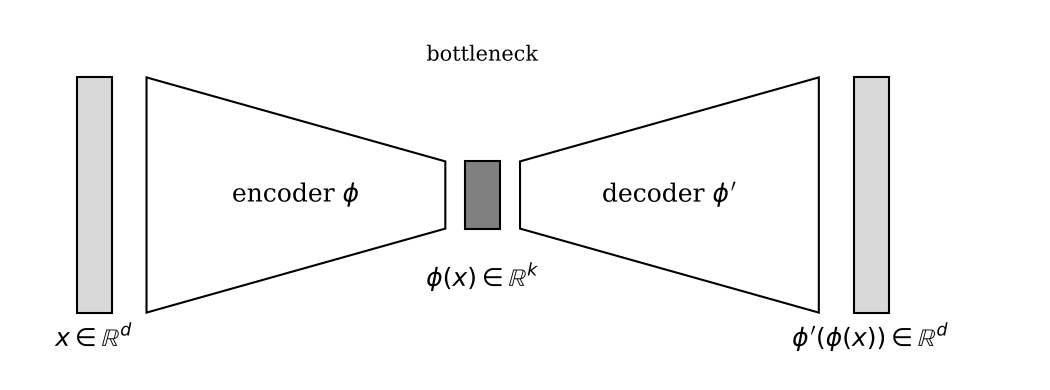
An autoencoder replaces PCA’s two matrices with two neural networks:
Training loss: reconstruction error, \[ \mathcal{L}(x_i) := \|x_i - \phi'(\phi(x_i))\|^2. \]
We pass each training point through the encoder and then the decoder, and compare the reconstruction with the original input. As always for neural networks, we train with SGD and backprop, so we only need the loss at a single data point. The encoder plays the role of \(U\) and the decoder the role of \(U^\top\). The two are trained together, but the encoder is what we use afterwards: to embed new data, we only need \(\phi(x)\), just as in PCA we only ever needed \(Ux\).
That’s really the whole idea. Today “autoencoder” refers to a whole class of architectures: anything that maps high-dimensional inputs to a lower dimension with a neural network, and back again with another one.
The first architecture called an autoencoder was introduced in 2006 for learning representations of images.
Read an architecture like an onion: start with the input and output, then look inside.
Every arrow without a label is a dense layer, so the parameter counts add up fast. The \(2000 \to 1000\) layer alone has a \(1000 \times 2000\) weight matrix, which is 2 million weights, plus 1,000 biases. All of these start out random and are learned from data.
Tied weights. The original autoencoder borrowed an idea from PCA: if the encoder uses a matrix \(W\) at some layer, the matching decoder layer uses \(W^\top\). Weights are usually not tied in modern autoencoders. The reason goes back to PCA. \(U^\top\) undoes \(U\) because \(U\) has orthonormal rows, and that interpretation doesn’t hold for a general matrix. An autoencoder’s encoder is a composition of unrestricted matrices and nonlinearities, so the transpose of its weights has no reason to be a good decoder. Since we don’t know how to write down the decoder for an arbitrary encoder, we let it be a separate network and learn it from the data.
The bottleneck dimension \(k\) is a hyperparameter that depends on what we want the embedding for. The uses are the same as for PCA. To visualize the data, choose \(k = 2\). A larger \(k\) might be used to remove noise while keeping the informative features, but that choice needs a justification from the application.
The 2006 paper compared the two methods on MNIST, the handwritten digits dataset. PCA projected the images to 2D, and a \(784\)–\(1000\)–\(500\)–\(250\)–\(2\) autoencoder embedded them into a 2-dimensional bottleneck. In a design like this, the first and last numbers (\(784\) and \(2\)) follow from the data and the task. Everything in between takes trial and error.
Both methods are unsupervised: the labels are not used to compute the embeddings and are only added as colors afterwards, to check whether the embedding makes sense. In the PCA embedding, only the 1s formed a clearly separate group. The autoencoder separated the digits much better. We reproduce this comparison in the coding example below.
You won’t need to implement backprop yourself in practice. Libraries such as PyTorch compute gradients for you. Here is the whole pipeline for training an autoencoder on MNIST (60,000 training images and 10,000 test images).
Mini-batches. In practice we use something between full gradient descent and single-example SGD. Mini-batch SGD computes the average gradient over a small batch of examples, such as 256, and then updates the parameters. It is still stochastic, because each step uses an estimate of the full gradient. With 60,000 training images and batch size 256, one pass through the data (an epoch) makes about \(60{,}000 / 256 \approx 235\) updates. Batch sizes are usually powers of 2, because computers handle them efficiently.
Build the autoencoder. We flatten each image from \(28 \times 28\) to a vector of length 784 and build a \(784\)–\(256\)–\(128\)–\(2\) autoencoder.
from torch import nn

encoder = nn.Sequential(
    nn.Flatten(),
    nn.Linear(28 * 28, 256), nn.ReLU(),
    nn.Linear(256, 128),     nn.ReLU(),
    nn.Linear(128, 2),
)

decoder = nn.Sequential(
    nn.Linear(2, 128),       nn.ReLU(),
    nn.Linear(128, 256),     nn.ReLU(),
    nn.Linear(256, 28 * 28),
    nn.Sigmoid(),                  # pixel values between 0 and 1
    nn.Unflatten(1, (1, 28, 28)),
)

autoencoder = nn.Sequential(encoder, decoder)
Each nn.Linear layer is exactly a dense layer from 4.1:
a weight matrix and a bias vector, to be learned. The final sigmoid
makes every output a number in \((0,
1)\), like a pixel intensity.
Loss and optimizer. Minimizing the reconstruction error is minimizing the mean squared error (MSE) between the reconstruction and the input. The optimizer decides how to use each gradient to update the parameters. Plain SGD subtracts a scaled gradient. Adam is a popular default that uses the gradients in a smarter way. You don’t need its details.
criterion = nn.MSELoss()
optimizer = torch.optim.Adam(autoencoder.parameters(), lr=1e-3)
Train. Each step processes one mini-batch. Notice that the labels are thrown away: each image is its own target.
for epoch in range(10):                 # 10 passes through the data
    for x, _ in train_loader:           # a mini-batch of 256 images, no labels
        optimizer.zero_grad()           # reset the gradient
        x_hat = autoencoder(x)          # forward pass
        loss = criterion(x_hat, x)      # compute the loss
        loss.backward()                 # backward pass: backprop computes the gradient
        optimizer.step()                # update the parameters using the gradient
loss.backward() is backprop: it computes the gradient of
the loss with respect to every parameter, the same calculation we did by
hand in 4.1.
Results. With plain SGD, the loss decreased only slowly. Switching to Adam, the training loss fell from 0.068 after the first epoch to 0.040 after ten, and the test loss tracked it closely, ending at 0.040.
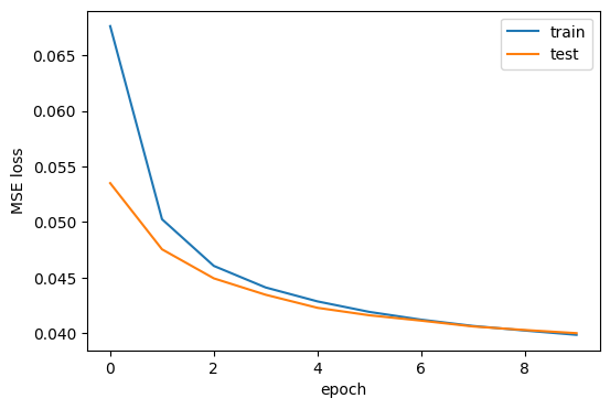
We track the test loss as well as the training loss because a network this flexible can keep driving the training loss down. If the test loss starts to go up while the training loss keeps falling, that is a sign to stop.
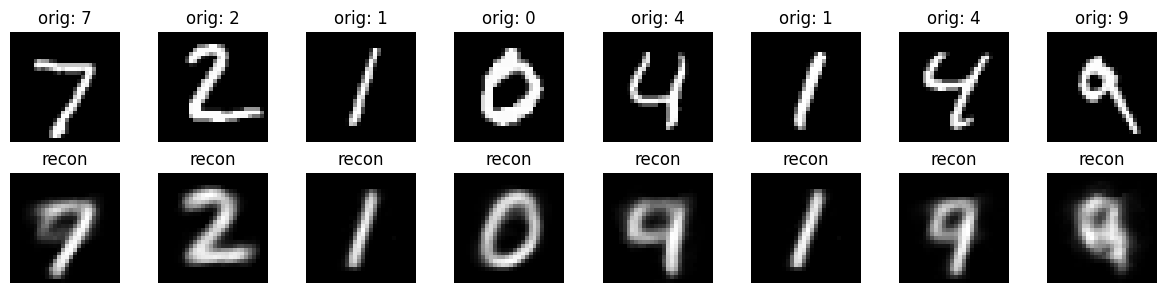
The reconstructions (bottom row) are blurry but recognizable, even though each image passed through just two numbers. The model sometimes confuses similar digits, such as 4 with 9 or 7 with 9.
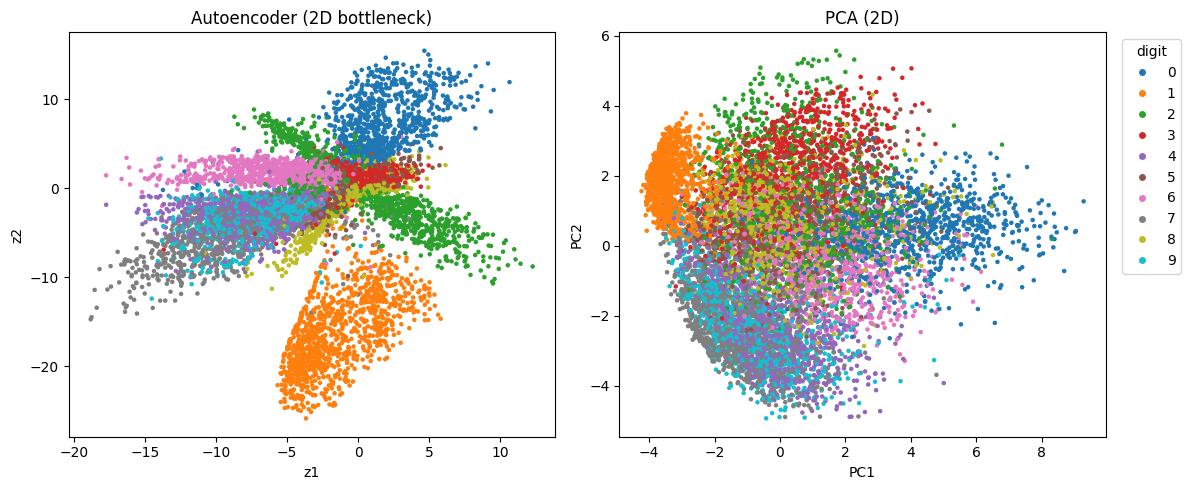
The 2D embeddings of the test set reproduce the paper’s finding. PCA (right) separates the 1s and mixes most other digits together. The autoencoder (left) keeps much more of the structure, with several digits forming their own regions. Our modern version, without tied weights, separates the digits even more clearly than the 2006 autoencoder did.
torch.optim.SGD instead of Adam and compare
the learning curves.Autoencoders have evolved over the past 20 years. Here are two important variants.
Goal: learn a representation that is robust against noise. Real data is often noisy, and we’d like a small amount of noise in the input not to change the learned representation much.
Idea: train an autoencoder to reconstruct clean inputs from corrupted ones.
\[ x \in \mathbb{R}^d \;\longrightarrow\; \tilde x \sim q(\tilde x \mid x) \;\xrightarrow{\text{ encoder } \phi\ }\; \phi(\tilde x) \in \mathbb{R}^k \;\xrightarrow{\text{ decoder } \phi'\ }\; \phi'(\phi(\tilde x)) \in \mathbb{R}^d \]
Training loss: reconstruction error, \[ \mathcal{L}(x_i) := \|x_i - \phi'(\phi(\tilde x_i))\|^2, \] where
The noise is added on the fly to each mini-batch during training. The network sees the corrupted input but is scored against the clean one. Denoising autoencoders aren’t widely used today, but the idea behind them, adding noise to data and training a model to recover the data, is the foundation of diffusion models, which power many modern image generators.
Question: what if we want to generate new data?
Idea: we already have a trained decoder. Sample points from \(\mathbb{R}^k\) (e.g. from \(N(0, I_k)\)), and pass the samples through the trained decoder.
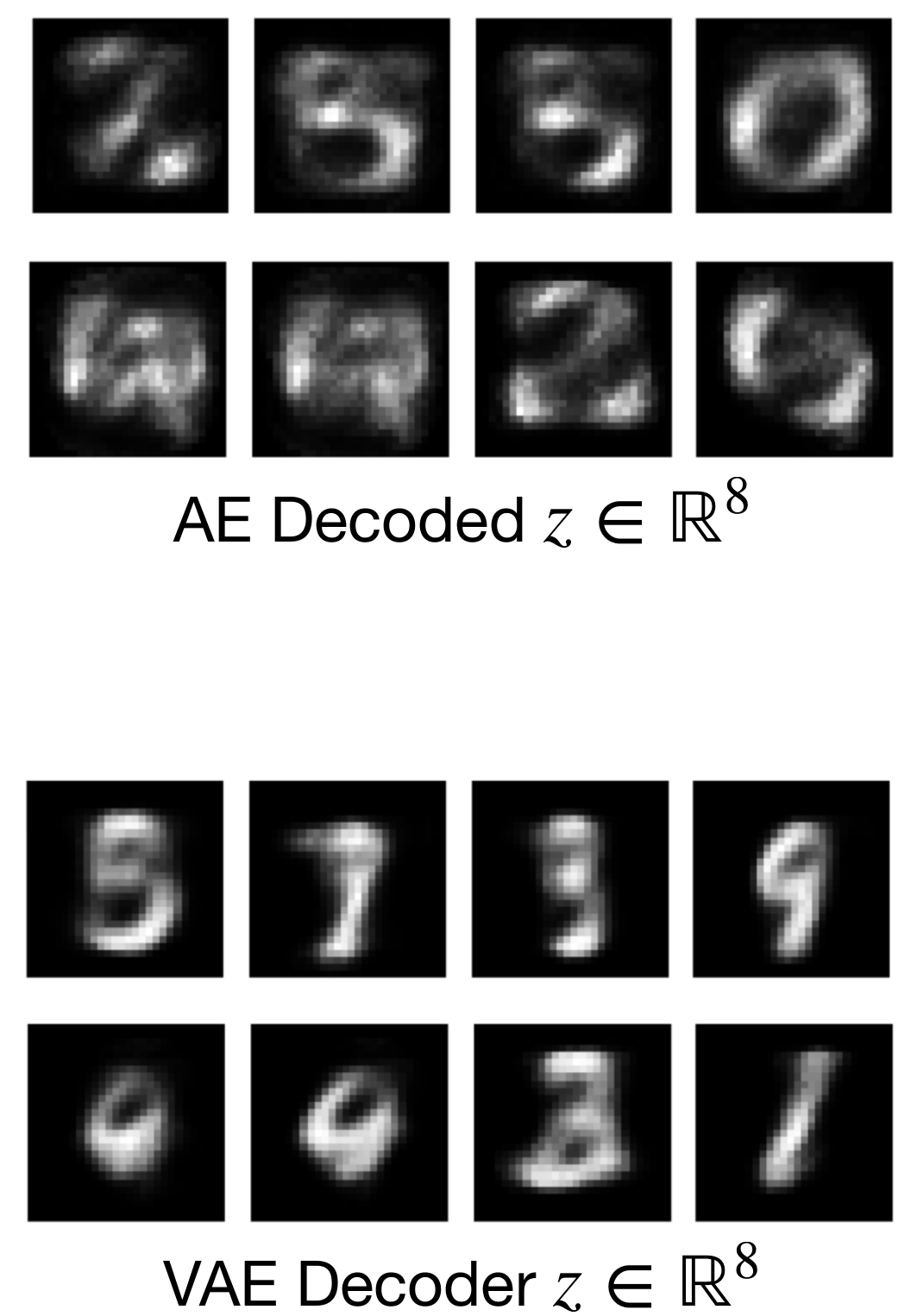
The top two rows show what this gives for an ordinary autoencoder with an 8-dimensional bottleneck, trained on MNIST. You can see digits in a few of them, but the quality is poor. The reason: nothing in the autoencoder’s training asks the encoded data to look like a Gaussian. Its only goal is reconstruction, so the encoded points can be spread out in a complicated way. Most samples from \(N(0, I_8)\) land where the decoder has never seen any data.
Goal (VAE): learn latent variables whose distribution is close to \(N(0, I_k)\).
If the encoded training data really is distributed like \(N(0, I_k)\), then sampling from \(N(0, I_k)\) and decoding should produce realistic images. The bottom two rows show samples from a VAE decoder with the same 8-dimensional latent space: they look much more like handwritten digits. Making this work takes more machinery than we have room for here, and VAEs are a good topic to read up on if you’re interested.